Filters-Instagram
This notebook includes both coding and written questions. Please hand in this notebook file with all the outputs and your answers to the written questions.
1 | # Setup |
2 | import numpy as np |
3 | import matplotlib.pyplot as plt |
4 | from time import time |
5 | #from skimage import io |
6 | |
7 | from __future__ import print_function |
8 | |
9 | %matplotlib inline |
10 | plt.rcParams['figure.figsize'] = (10.0, 8.0) # set default size of plots |
11 | plt.rcParams['image.interpolation'] = 'nearest' |
12 | plt.rcParams['image.cmap'] = 'gray' |
13 | |
14 | # for auto-reloading extenrnal modules |
15 | %load_ext autoreload |
16 | %autoreload 2 |
Convolutions
@(Commutative Property)
Recall that the convolution of an image and a kernel is defined as follows:
将式中积分变量 i 和 j 置换为 m−x 和 n−y,即可证明
@(Linear and Shift Invariance)
Let be a function . Consider a system , where with some kernel . Show that defined by any kernel is a Linear Shift Invariant (LSI) system. In other words, for any , show that satisfies both of the following:
向量化
向量化可以提高计算效率,实现更快的卷积计算。
向量化的思路就是:
- 将卷积核进行向量化
- 将迭代过程中的计算块(计算中心及其领域)进行向量化,由于运算的对象都是核,此处可以将向量化的计算块拼成矩阵
- 两者进行内积计算,并reshape成原有图像大小
Cross-correlation
Cross-correlation of two 2D signals and is defined as follows:
Template Matching with Cross-correlation
使用互相关性实现模板匹配
Suppose that you are a clerk at a grocery store. One of your responsibilites is to check the shelves periodically and stock them up whenever there are sold-out items. You got tired of this laborious task and decided to build a computer vision system that keeps track of the items on the shelf.
Luckily, you have learned in CS131 that cross-correlation can be used for template matching: a template is multiplied with regions of a larger image to measure how similar each region is to the template.
The template of a product (template.jpg) and the image of shelf (shelf.jpg) is provided. We will use cross-correlation to find the product in the shelf.
Implement cross_correlation function in filters.py and run the code below.Hint: you may use the conv_fast function you implemented in the previous question.
1 | from filters import cross_correlation |
2 | |
3 | # Load template and image in grayscale |
4 | img = io.imread('shelf.jpg') |
5 | img_grey = io.imread('shelf.jpg', as_grey=True) |
6 | temp = io.imread('template.jpg') |
7 | temp_grey = io.imread('template.jpg', as_grey=True) |
8 | |
9 | # Perform cross-correlation between the image and the template |
10 | out = cross_correlation(img_grey, temp_grey) |
11 | |
12 | # Find the location with maximum similarity |
13 | y,x = (np.unravel_index(out.argmax(), out.shape)) |
14 | |
15 | # Display product template |
16 | plt.figure(figsize=(25,20)) |
17 | plt.subplot(3, 1, 1) |
18 | plt.imshow(temp) |
19 | plt.title('Template') |
20 | plt.axis('off') |
21 | |
22 | # Display cross-correlation output |
23 | plt.subplot(3, 1, 2) |
24 | plt.imshow(out) |
25 | plt.title('Cross-correlation (white means more correlated)') |
26 | plt.axis('off') |
27 | |
28 | # Display image |
29 | plt.subplot(3, 1, 3) |
30 | plt.imshow(img) |
31 | plt.title('Result (blue marker on the detected location)') |
32 | plt.axis('off') |
33 | |
34 | # Draw marker at detected location |
35 | plt.plot(x, y, 'bx', ms=40, mew=10) |
36 | plt.show() |
Interpretation
How does the output of cross-correlation filter look like? Was it able to detect the product correctly? Explain what might be the problem with using raw template as a filter.
Zero-mean cross-correlation
A solution to this problem is to subtract off the mean value of the template so that it has zero mean.
Implement zero_mean_cross_correlation function in filters.py and run the code below.
Normalized Cross-correlation
One day the light near the shelf goes out and the product tracker starts to malfunction. The zero_mean_cross_correlation is not robust to change in lighting condition. The code below demonstrates this.
A solution is to normalize the pixels of the image and template at every step before comparing them. This is called normalized cross-correlation.
The mathematical definition for normalized cross-correlation of and template is:
where
is the patch image at position (m,n)
is the mean of the patch image
is the standard deviation of the patch image
is the mean of the template
is the standard deviation of the template
不可以直接对整幅待匹配的图做归一化操作。
正确的图像区域,如果是做整幅图的归一化,明显受到了其他区域诸如亮度颜色等的影响,干扰了匹配。
应该对每个待匹配块做归一化操作,然后比较匹配程度。
Separable Filters
Consider a image I and a filter F. A filter F is separable if it can be written as a product of two 1D filters: .
For example,
can be written as a matrix product of
Therefore is a separable filter.
For any separable filter
Complexity comparison
- 乘法操作的次数为
- 乘法操作的次数为
Edges-Smart Car Lane Detection
Canny Edge Detector
In this part, you are going to implment Canny edge detector. The Canny edge detection algorithm can be broken down in to five steps:
- Smoothing:平滑处理(去躁)
- Finding gradients:寻找梯度
- Non-maximum suppression:非极大值抑制
- Double thresholding:双阈值算法
- Edge tracking by hysteresis:滞后边缘追踪
Smoothing
We first smooth the input image by convolving it with a Gaussian kernel. The equation for a Gaussian kernel of size (2k+1)×(2k+1) is given by:
Implement gaussian_kernel in edge.py and run the code below.
1 | from edge import conv, gaussian_kernel |
2 | |
3 | # Define 3x3 Gaussian kernel with std = 1 |
4 | kernel = gaussian_kernel(3, 1) |
5 | kernel_test = np.array( |
6 | [[ 0.05854983, 0.09653235, 0.05854983], |
7 | [ 0.09653235, 0.15915494, 0.09653235], |
8 | [ 0.05854983, 0.09653235, 0.05854983]] |
9 | ) |
10 | # print(kernel) |
11 | |
12 | # Test Gaussian kernel |
13 | if not np.allclose(kernel, kernel_test): |
14 | print('Incorrect values! Please check your implementation.') |
需要先实现edge.py中的conv卷积函数,可以使用作业hw1中的conv_nested,conv_fast,conv_faster等函数
1 | # Test with different kernel_size and sigma |
2 | kernel_size = 5 |
3 | sigma = 1.4 |
4 | |
5 | # Load image |
6 | img = io.imread('iguana.png', as_grey=True) |
7 | |
8 | # Define 5x5 Gaussian kernel with std = sigma |
9 | kernel = gaussian_kernel(kernel_size, sigma) |
10 | |
11 | # Convolve image with kernel to achieve smoothed effect |
12 | smoothed = conv(img, kernel) |
13 | |
14 | plt.subplot(1,2,1) |
15 | plt.imshow(img) |
16 | plt.title('Original image') |
17 | plt.axis('off') |
18 | |
19 | plt.subplot(1,2,2) |
20 | plt.imshow(smoothed) |
21 | plt.title('Smoothed image') |
22 | plt.axis('off') |
23 | |
24 | plt.show() |
What is the effect of the kernel_size and sigma?
高斯滤波器用像素邻域的加权均值来代替该点的像素值,而每一邻域像素点权值是随该点与中心点的距离单调增减的,因为边缘是一种图像局部特征,如果平滑运算对离算子中心很远的像素点仍然有很大作用,则平滑运算会使图像失真。
高斯滤波器宽度(决定着平滑程度)是由参数σ表征的,而且σ和平滑程度的关系是非常简单的.σ越大,高斯滤波器的频带就越宽,平滑程度就越好.通过调节平滑程度参数σ,可在图像特征过分模糊(过平滑)与平滑图像中由于噪声和细纹理所引起的过多的不希望突变量(欠平滑)之间取得折衷。
Finding gradients
The gradient of a 2D scalar function in Cartesian coordinate is defined by:
Note that the partial derivatives can be computed by convolving the image with some appropriate kernels and :
Find the kernels and and implement partial_x and partial_y using conv defined in edge.py.
-Hint: Remeber that convolution flips the kernel.
1 | from edge import partial_x, partial_y |
2 | |
3 | # Test input |
4 | I = np.array( |
5 | [[0, 0, 0], |
6 | [0, 1, 0], |
7 | [0, 0, 0]] |
8 | ) |
9 | |
10 | # Expected outputs |
11 | I_x_test = np.array( |
12 | [[ 0, 0, 0], |
13 | [ 0.5, 0, -0.5], |
14 | [ 0, 0, 0]] |
15 | ) |
16 | |
17 | I_y_test = np.array( |
18 | [[ 0, 0.5, 0], |
19 | [ 0, 0, 0], |
20 | [ 0, -0.5, 0]] |
21 | ) |
22 | |
23 | # Compute partial derivatives |
24 | I_x = partial_x(I) |
25 | I_y = partial_y(I) |
26 | |
27 | # Test correctness of partial_x and partial_y |
28 | if not np.all(I_x == I_x_test): |
29 | print('partial_x incorrect') |
30 | |
31 | if not np.all(I_y == I_y_test): |
32 | print('partial_y incorrect') |
1 | # Compute partial derivatives of smoothed image |
2 | Gx = partial_x(smoothed) |
3 | Gy = partial_y(smoothed) |
4 | |
5 | plt.subplot(1,2,1) |
6 | plt.imshow(Gx) |
7 | plt.title('Derivative in x direction') |
8 | plt.axis('off') |
9 | |
10 | plt.subplot(1,2,2) |
11 | plt.imshow(Gy) |
12 | plt.title('Derivative in y direction') |
13 | plt.axis('off') |
14 | |
15 | plt.show() |
What is the reason for performing smoothing prior to computing the gradients?
平滑是为了去噪,噪声会使得计算梯度时得到幅度较大的异常值。
Now, we can compute the magnitude and direction of gradient with the two partial derivatives:
Implement gradient in
edge.pywhich takes in an image and outputs and .
1 | from edge import gradient |
2 | |
3 | G, theta = gradient(smoothed) |
4 | |
5 | if not np.all(G >= 0): |
6 | print('Magnitude of gradients should be non-negative.') |
7 | |
8 | if not np.all((theta >= 0) * (theta < 360)): |
9 | print('Direction of gradients should be in range 0 <= theta < 360') |
10 | |
11 | plt.imshow(G) |
12 | plt.title('Gradient magnitude') |
13 | plt.axis('off') |
14 | plt.show() |
Non-maximum suppression
You should be able to note that the edges extracted from the gradient of the smoothed image is quite thick and blurry. The purpose of this step is to convert the “blurred” edges into “sharp” edges. Basically, this is done by preserving all local maxima in the gradient image and discarding everything else. The algorithm is for each pixel in the gradient image:
- Round the gradient direction to the nearest 45 degrees, corresponding to the use of an 8-connected neighbourhood.
当然这种做法其实是简化版本的,虽然Canny的论文上是这么写的,但是后来也有提出,梯度肯定不止这四个,针对别的梯度方向的比较,使用插值等方法来进行非极大值抑制. Canny算子中的非极大值抑制(Non-Maximum Suppression)分析
- Compare the edge strength of the current pixel with the edge strength of the pixel in the positive and negative gradient direction. For example, if the gradient direction is south (theta=90), compare with the pixels to the north and south.
- If the edge strength of the current pixel is the largest; preserve the value of the edge strength. If not, suppress (i.e. remove) the value.
非极大值抑制属于一种边缘细化的方法,梯度大的位置有可能为边缘,在这些位置沿着梯度方向,找到像素点的局部最大值,并将其非最大值抑制。
形象的说就是一条粗粗的区域都根据梯度强度判断成了边缘,但目标只需要一条细细的边,这个时候就找区域内的最大的那条作为边(注意是沿着梯度方向),其他的或抛弃或作为备选区域
1 | from edge import non_maximum_suppression |
2 | |
3 | nms = non_maximum_suppression(G, theta) |
4 | plt.imshow(nms) |
5 | plt.title('Non-maximum suppressed') |
6 | plt.axis('off') |
7 | plt.show() |
Double Thresholding
The edge-pixels remaining after the non-maximum suppression step are (still) marked with their strength pixel-by-pixel. Many of these will probably be true edges in the image, but some may be caused by noise or color variations, for instance, due to rough surfaces. The simplest way to discern between these would be to use a threshold, so that only edges stronger that a certain value would be preserved. The Canny edge detection algorithm uses double thresholding. Edge pixels stronger than the high threshold are marked as strong; edge pixels weaker than the low threshold are suppressed and edge pixels between the two thresholds are marked as weak.
Implement double_thresholding in edge.py
双阀值方法,设置一个maxval,以及minval,梯度大于maxval则为强边缘,梯度值介于maxval与minval则为弱边缘点,小于minval为抑制点。
双阈值的结果在第五步可以用来作为边缘追踪的依据。
1 | from edge import double_thresholding |
2 | |
3 | low_threshold = 0.02 |
4 | high_threshold = 0.03 |
5 | |
6 | strong_edges, weak_edges = double_thresholding(nms, high_threshold, low_threshold) |
7 | assert(np.sum(strong_edges & weak_edges) == 0) |
8 | |
9 | edges=strong_edges * 1.0 + weak_edges * 0.5 |
10 | |
11 | plt.subplot(1,2,1) |
12 | plt.imshow(strong_edges) |
13 | plt.title('Strong Edges') |
14 | plt.axis('off') |
15 | |
16 | plt.subplot(1,2,2) |
17 | plt.imshow(edges) |
18 | plt.title('Strong+Weak Edges') |
19 | plt.axis('off') |
20 | |
21 | plt.show() |
Edge tracking
Strong edges are interpreted as “certain edges”, and can immediately be included in the final edge image. Weak edges are included if and only if they are connected to strong edges. The logic is of course that noise and other small variations are unlikely to result in a strong edge (with proper adjustment of the threshold levels). Thus strong edges will (almost) only be due to true edges in the original image. The weak edges can either be due to true edges or noise/color variations. The latter type will probably be distributed in dependently of edges on the entire image, and thus only a small amount will be located adjacent to strong edges. Weak edges due to true edges are much more likely to be connected directly to strong edges.
Implement link_edges in edge.py
由于边缘是连续的,因此可以认为弱边缘如果为真实边缘则和强边缘是联通的,可由此判断其是否为真实边缘。
Canny edge detector
Implement canny in edge.py using the functions you have implemented so far. Test edge detector with different parameters.
1 | from edge import canny |
2 | |
3 | # Load image |
4 | img = io.imread('iguana.png', as_grey=True) |
5 | |
6 | # Run Canny edge detector |
7 | edges = canny(img, kernel_size=5, sigma=1.4, high=0.04, low=0.02) |
8 | print (edges.shape) |
9 | plt.imshow(edges) |
10 | plt.axis('off') |
11 | plt.show() |
Suppose that the Canny edge detector successfully detects an edge in an image. The edge is then rotated by , where the relationship between a point on the original edge and a point on the rotated edge is defined as
Will the rotated edge be detected using the same Canny edge detector? Provide either a mathematical proof or a counter example.
-Hint: The detection of an edge by the Canny edge detector depends only on the magnitude of its derivative. The derivative at point is determined by its components along the and directions. Think about how these magnitudes have changed because of the rotation.
幅度没变,所以边缘检测不变。
After running the Canny edge detector on an image, you notice that long edges are broken into short segments separated by gaps. In addition, some spurious edges appear. For each of the two thresholds (low and high) used in hysteresis thresholding, explain how you would adjust the threshold (up or down) to address both problems. Assume that a setting exists for the two thresholds that produces the desired result. Briefly explain your answer.
调参方法:
如果长直线被断成小段,说明weak_edges的阈值太大,weak_edges的数量较少,此时应当调低weak_edges的阈值。
如果spurious (伪直线)出现,说明strong_edges的阈值太小,strong_edges的数量较多,此时应当调高strong_edges的阈值。
Extra Credit: Optimizing Edge Detector
One way of evaluating an edge detector is to compare detected edges with manually specified ground truth edges. Here, we use precision, recall and F1 score as evaluation metrics. We provide you 40 images of objects with ground truth edge annotations. Run the code below to compute precision, recall and F1 score over the entire set of images. Then, tweak the parameters of the Canny edge detector to get as high F1 score as possible. You should be able to achieve F1 score higher than 0.31 by carefully setting the parameters.
1 | from os import listdir |
2 | from itertools import product |
3 | |
4 | # Define parameters to test |
5 | sigmas = [1.6, 1.7, 1.8, 1.9, 2.0] |
6 | highs = [0.04, 0.05, 0.06] |
7 | lows = [0.015, 0.02, 0.025] |
8 | |
9 | for sigma, high, low in product(sigmas, highs, lows): |
10 | |
11 | print("sigma={}, high={}, low={}".format(sigma, high, low)) |
12 | n_detected = 0.0 |
13 | n_gt = 0.0 |
14 | n_correct = 0.0 |
15 | |
16 | for img_file in listdir('images/objects'): |
17 | img = io.imread('images/objects/'+img_file, as_grey=True) |
18 | gt = io.imread('images/gt/'+img_file+'.gtf.pgm', as_grey=True) |
19 | |
20 | mask = (gt != 5) # 'don't' care region |
21 | gt = (gt == 0) # binary image of GT edges |
22 | |
23 | edges = canny(img, kernel_size=5, sigma=sigma, high=high, low=low) |
24 | edges = edges * mask |
25 | |
26 | n_detected += np.sum(edges) |
27 | n_gt += np.sum(gt) |
28 | n_correct += np.sum(edges * gt) |
29 | |
30 | p_total = n_correct / n_detected |
31 | r_total = n_correct / n_gt |
32 | f1 = 2 * (p_total * r_total) / (p_total + r_total) |
33 | print('Total precision={:.4f}, Total recall={:.4f}'.format(p_total, r_total)) |
34 | print('F1 score={:.4f}'.format(f1)) |
Lane Detection
In this section we will implement a simple lane detection application using Canny edge detector and Hough transform.
Here are some example images of how your final lane detector will look like.
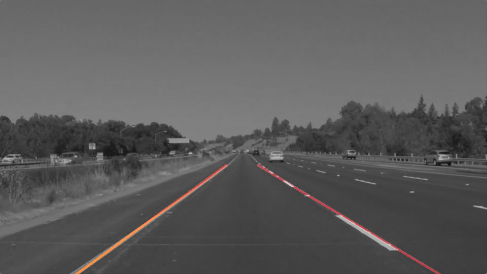
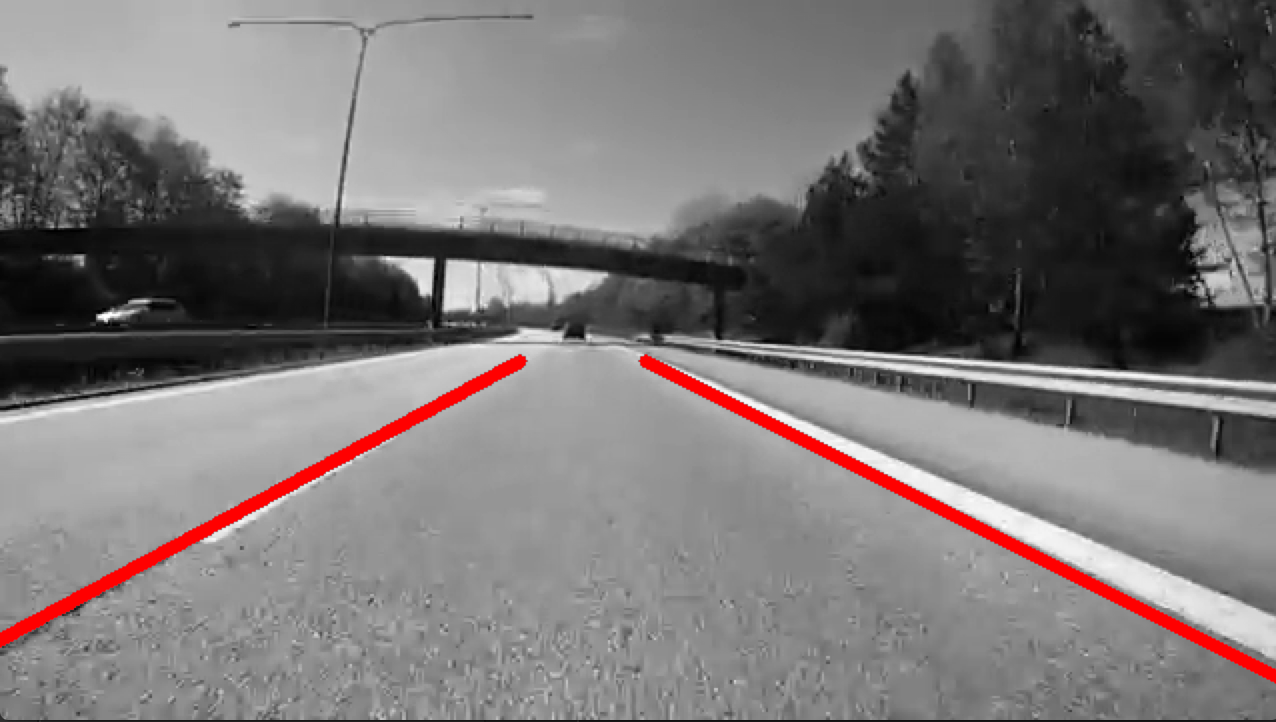
The algorithm can broken down into the following steps:
- Detect edges using the Canny edge detector.
- Extract the edges in the region of interest (a triangle covering the bottom corners and the center of the image).
- Run Hough transform to detect lanes.
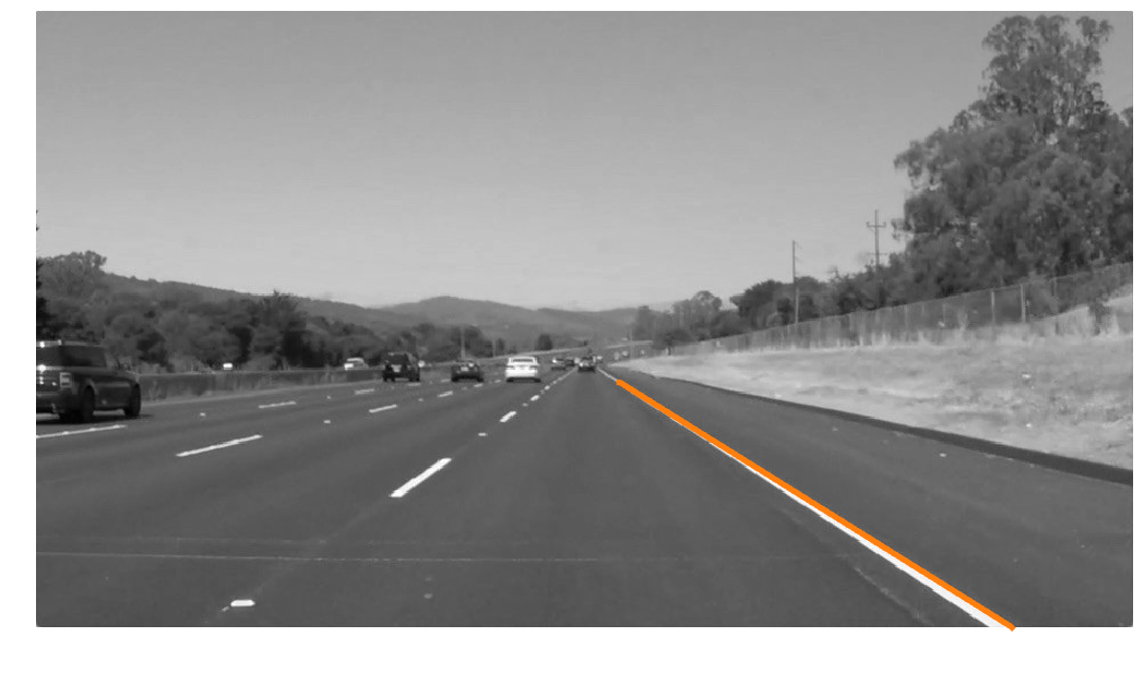
Edge detection
Lanes on the roads are usually thin and long lines with bright colors. Our edge detection algorithm by itself should be able to find the lanes pretty well. Run the code cell below to load the example image and detect edges from the image.
1 | from edge import canny |
2 | |
3 | # Load image |
4 | img = io.imread('road.jpg', as_grey=True) |
5 | |
6 | # Run Canny edge detector |
7 | edges = canny(img, kernel_size=5, sigma=1.4, high=0.03, low=0.008) |
8 | |
9 | |
10 | plt.subplot(211) |
11 | plt.imshow(img) |
12 | plt.axis('off') |
13 | plt.title('Input Image') |
14 | |
15 | plt.subplot(212) |
16 | plt.imshow(edges) |
17 | plt.axis('off') |
18 | plt.title('Edges') |
19 | plt.show() |
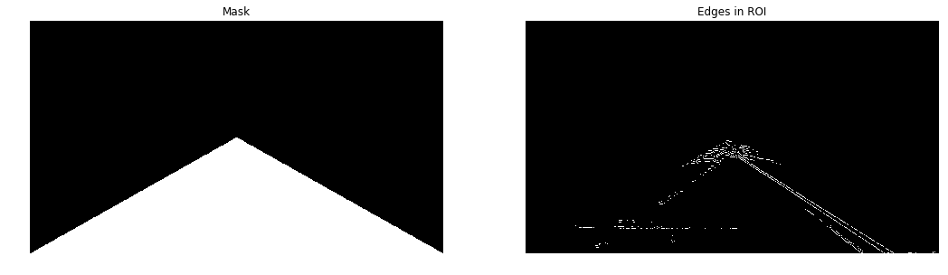
Extracting region of interest (ROI)
We can see that the Canny edge detector could find the edges of the lanes. However, we can also see that there are edges of other objects that we are not interested in. Given the position and orientation of the camera, we know that the lanes will be located in the lower half of the image. The code below defines a binary mask for the ROI and extract the edges within the region.
1 | H, W = img.shape |
2 | |
3 | # Generate mask for ROI (Region of Interest) |
4 | mask = np.zeros((H, W)) |
5 | for i in range(H): |
6 | for j in range(W): |
7 | if i > (H / W) * j and i > -(H / W) * j + H: |
8 | mask[i, j] = 1 |
9 | |
10 | # Extract edges in ROI |
11 | roi = edges * mask |
12 | |
13 | plt.subplot(1,2,1) |
14 | plt.imshow(mask) |
15 | plt.title('Mask') |
16 | plt.axis('off') |
17 | |
18 | plt.subplot(1,2,2) |
19 | plt.imshow(roi) |
20 | plt.title('Edges in ROI') |
21 | plt.axis('off') |
22 | plt.show() |
Fitting lines using Hough transform
The output from the edge detector is still a collection of connected points. However, it would be more natural to represent a lane as a line parameterized as , with a slope and -intercept . We will use Hough transform to find parameterized lines that represent the detected edges.
In general, a straight line can be represented as a point in the parameter space. However, this cannot represent vertical lines as the slope parameter will be unbounded. Alternatively, we parameterize a line using and as follows:
Using this parameterization, we can map everypoint in -space to a sine-like line in -space (or Hough space). We then accumulate the parameterized points in the Hough space and choose points (in Hough space) with highest accumulated values. A point in Hough space then can be transformed back into a line in -space.
See lectures on Hough transform.
Implement hough_transform in edge.py.
1 | from edge import hough_transform |
2 | |
3 | # Perform Hough transform on the ROI |
4 | acc, rhos, thetas = hough_transform(roi) |
5 | |
6 | # Coordinates for right lane |
7 | xs_right = [] |
8 | ys_right = [] |
9 | |
10 | # Coordinates for left lane |
11 | xs_left = [] |
12 | ys_left = [] |
13 | |
14 | for i in range(20): |
15 | idx = np.argmax(acc) |
16 | r_idx = idx // acc.shape[1] |
17 | t_idx = idx % acc.shape[1] |
18 | acc[r_idx, t_idx] = 0 # Zero out the max value in accumulator |
19 | |
20 | rho = rhos[r_idx] |
21 | theta = thetas[t_idx] |
22 | |
23 | # Transform a point in Hough space to a line in xy-space. |
24 | a = - (np.cos(theta)/np.sin(theta)) # slope of the line |
25 | b = (rho/np.sin(theta)) # y-intersect of the line |
26 | |
27 | # Break if both right and left lanes are detected |
28 | if xs_right and xs_left: |
29 | break |
30 | |
31 | if a < 0: # Left lane |
32 | if xs_left: |
33 | continue |
34 | xs = xs_left |
35 | ys = ys_left |
36 | else: # Right Lane |
37 | if xs_right: |
38 | continue |
39 | xs = xs_right |
40 | ys = ys_right |
41 | |
42 | for x in range(img.shape[1]): |
43 | y = a * x + b |
44 | if y > img.shape[0] * 0.6 and y < img.shape[0]: |
45 | xs.append(x) |
46 | ys.append(int(round(y))) |
47 | |
48 | plt.imshow(img) |
49 | plt.plot(xs_left, ys_left, linewidth=5.0) |
50 | plt.plot(xs_right, ys_right, linewidth=5.0) |
51 | plt.axis('off') |
52 | plt.show() |
之所以只检测出一条直线,是因为上面的边缘检测部分不是很完美,尤其是左边车道线的边缘检测出现了问题,才会导致左边车道线做霍夫变换也得不到理想的结果
Panorama-ImageStiching
This assignment covers Harris corner detector(角点检测器), RANSAC(随机抽样一致) and HOG descriptor(HOG描述子).
Panorama stitching is an early success of computer vision. Matthew Brown and David G. Lowe published a famous panoramic image stitching paper in 2007. Since then, automatic panorama stitching technology has been widely adopted in many applications such as Google Street View, panorama photos on smartphones,and stitching software such as Photosynth and AutoStitch.
In this assignment, we will detect and match keypoints from multiple images to build a single panoramic image. This will involve several tasks:
- Use Harris corner detector to find keypoints.
- Build a descriptor to describe each point in an image.
Compare two sets of descriptors coming from two different images and find matching keypoints.- Given a list of matching keypoints, use least-squares method to find the affine transformation matrix that maps points in one image to another.
- Use RANSAC to give a more robust estimate of affine transformation matrix.
Given the transformation matrix, use it to transform the second image and overlay it on the first image, forming a panorama.- Implement a different descriptor (HOG descriptor) and get another stitching result.
Harris Corner Detector
In this section, you are going to implement Harris corner detector for keypoint localization. Review the lecture slides on Harris corner detector to understand how it works. The Harris detection algorithm can be divide into the following steps:
- Compute and derivatives of an image
- Compute products of derivatives () at each pixel
- Compute matrix M at each pixel, where
- Compute corner response at each pixel
- Output corner response map
Step 1 is already done for you in the function harris_corners in panorama.py. Complete the function implementation and run the code below.
-Hint: You may use the function
scipy.ndimage.filters.convolve, which is already imported inpanoramy.py
关于Harris角点检测,这里有篇博客总结的很好。Harris角点
1 | from panorama import harris_corners |
2 | |
3 | img = imread('sudoku.png', as_grey=True) |
4 | |
5 | # Compute Harris corner response |
6 | response = harris_corners(img) |
7 | |
8 | # Display corner response |
9 | plt.subplot(1,2,1) |
10 | plt.imshow(response) |
11 | plt.axis('off') |
12 | plt.title('Harris Corner Response') |
13 | |
14 | plt.subplot(1,2,2) |
15 | plt.imshow(imread('solution_harris.png', as_grey=True)) |
16 | plt.axis('off') |
17 | plt.title('Harris Corner Solution') |
18 | |
19 | plt.show() |
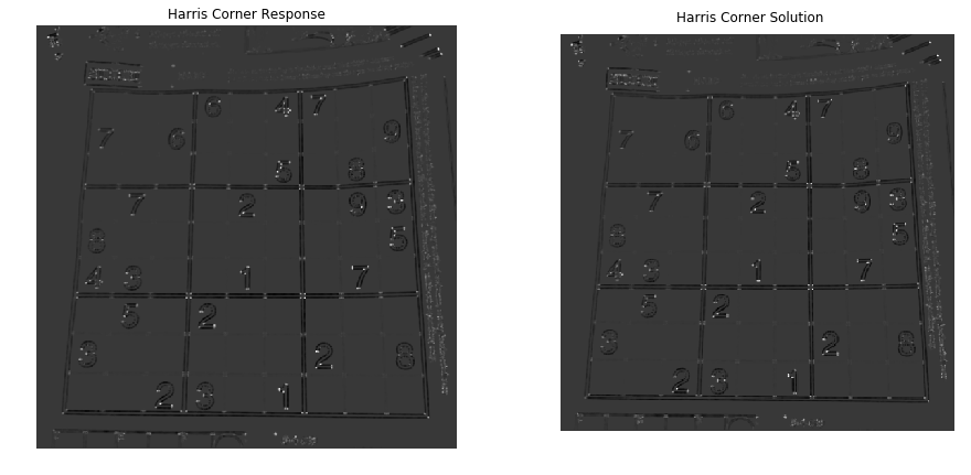
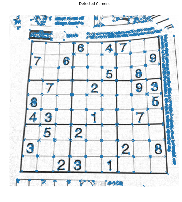
Once you implement the Harris detector correctly, you will be able to see small bright blobs around the corners of the sudoku grids and letters in the output corner response image. The function corner_peaks from skimage.feature performs non-maximum suppression to take local maxima of the response map and localize keypoints.
对响应输出进行非极大抑制。
1 | # Perform non-maximum suppression in response map |
2 | # and output corner coordiantes |
3 | corners = corner_peaks(response, threshold_rel=0.01) |
4 | |
5 | # Display detected corners |
6 | plt.imshow(img) |
7 | plt.scatter(corners[:,1], corners[:,0], marker='x') |
8 | plt.axis('off') |
9 | plt.title('Detected Corners') |
10 | plt.show() |
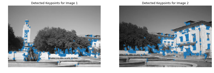
Describing and Matching Keypoints
We are now able to localize keypoints in two images by running the Harris corner detector independently on them. Next question is, how do we determine which pair of keypoints come from corresponding locations in those two images? In order to match the detected keypoints, we must come up with a way to describe the keypoints based on their local appearance. Generally, each region around detected keypoint locations is converted into a fixed-size vectors called descriptors.
Creating Descriptors
In this section, you are going to implement a simple_descriptor; each keypoint is described by normalized intensity in a small patch around it.
为了进行两幅图像中的关键点的点与点之间的匹配,需要对关键点进行描述。
此时,提出描述符对关键点的局部特征进行描述。
一般来说,描述符就是将检测到的关键点的附近区域转换成固定大小的向量。
1 | from panorama import harris_corners |
2 | |
3 | img1 = imread('uttower1.jpg', as_grey=True) |
4 | img2 = imread('uttower2.jpg', as_grey=True) |
5 | |
6 | # Detect keypoints in two images |
7 | keypoints1 = corner_peaks(harris_corners(img1, window_size=3), |
8 | threshold_rel=0.05, |
9 | exclude_border=8) |
10 | keypoints2 = corner_peaks(harris_corners(img2, window_size=3), |
11 | threshold_rel=0.05, |
12 | exclude_border=8) |
13 | |
14 | # Display detected keypoints |
15 | plt.subplot(1,2,1) |
16 | plt.imshow(img1) |
17 | plt.scatter(keypoints1[:,1], keypoints1[:,0], marker='x') |
18 | plt.axis('off') |
19 | plt.title('Detected Keypoints for Image 1') |
20 | |
21 | plt.subplot(1,2,2) |
22 | plt.imshow(img2) |
23 | plt.scatter(keypoints2[:,1], keypoints2[:,0], marker='x') |
24 | plt.axis('off') |
25 | plt.title('Detected Keypoints for Image 2') |
26 | plt.show() |
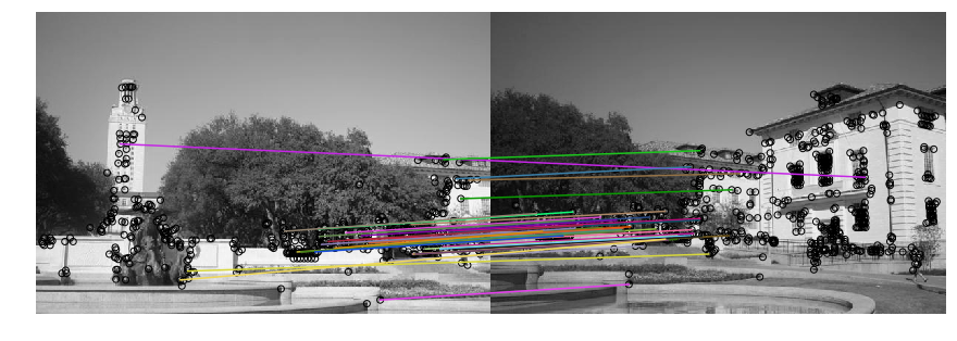
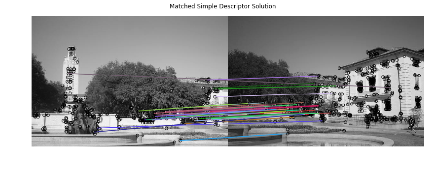
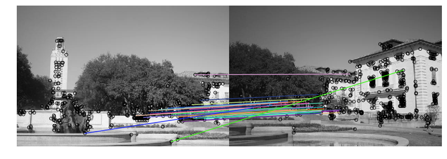
Matching Descriptors
Then, implement match_descriptors function to find good matches in two sets of descriptors. First, calculate Euclidean distance between all pairs of descriptors from image 1 and image 2. Then use this to determine if there is a good match: if the distance to the closest vector is significantly (by a factor which is given) smaller than the distance to the second-closest, we call it a match. The output of the function is an array where each row holds the indices of one pair of matching descriptors.
- 使用标准化的密度来作为描述子
- 使用欧几里得距离来对描述子进行匹配,当最短距离与第二短距离的比值小于阈值,则判定为匹配
1 | from panorama import simple_descriptor, match_descriptors, describe_keypoints |
2 | from utils import plot_matches |
3 | |
4 | patch_size = 5 |
5 | |
6 | # Extract features from the corners |
7 | desc1 = describe_keypoints(img1, keypoints1, |
8 | desc_func=simple_descriptor, |
9 | patch_size=patch_size) |
10 | desc2 = describe_keypoints(img2, keypoints2, |
11 | desc_func=simple_descriptor, |
12 | patch_size=patch_size) |
13 | |
14 | # Match descriptors in image1 to those in image2 |
15 | matches = match_descriptors(desc1, desc2, 0.7) |
16 | |
17 | # Plot matches |
18 | fig, ax = plt.subplots(1, 1, figsize=(15, 12)) |
19 | ax.axis('off') |
20 | plot_matches(ax, img1, img2, keypoints1, keypoints2, matches) |
21 | plt.show() |
22 | plt.imshow(imread('solution_simple_descriptor.png')) |
23 | plt.axis('off') |
24 | plt.title('Matched Simple Descriptor Solution') |
25 | plt.show() |
Transformation Estimation
We now have a list of matched keypoints across the two images. We will use this to find a transformation matrix that maps points in the second image to the corresponding coordinates in the first image. In other words, if the point in image 1 matches with in image 2, we need to find an affine transformation matrix H such that
\tilde {p_2} H = \tilde{p_1}$$ where $\tilde {p_1}, \tilde{p_2}$ are homogenous coordinates of $p_1$ and $p_2$.
Note that it may be impossible to find the transformation that maps every point in image 2 exactly to the corresponding point in image 1. However, we can estimate the transformation matrix with least squares. Given N matched keypoint pairs, let and be matrices whose rows are homogenous coordinates of corresponding keypoints in image 1 and image 2 respectively. Then, we can estimate H by solving the least squares problem
Implement fit_affine_matrix in panorama.py
-Hint: read the documentation about np.linalg.lstsq
第三步就是要计算图2到图1的仿射变换矩阵。
由于匹配点对众多,这里采用最小二乘法估计变换矩阵。
1 | from panorama import fit_affine_matrix |
2 | |
3 | # Sanity check for fit_affine_matrix |
4 | |
5 | # Test inputs |
6 | a = np.array([[0.5, 0.1], [0.4, 0.2], [0.8, 0.2]]) |
7 | b = np.array([[0.3, -0.2], [-0.4, -0.9], [0.1, 0.1]]) |
8 | |
9 | H = fit_affine_matrix(b, a) |
10 | |
11 | # Target output |
12 | sol = np.array( |
13 | [[1.25, 2.5, 0.0], |
14 | [-5.75, -4.5, 0.0], |
15 | [0.25, -1.0, 1.0]] |
16 | ) |
17 | |
18 | error = np.sum((H - sol) ** 2) |
19 | |
20 | if error < 1e-20: |
21 | print('Implementation correct!') |
22 | else: |
23 | print('There is something wrong.') |
After checking that your fit_affine_matrix function is running correctly, run the following code to apply it to images.
Images will be warped and image 2 will be mapped to image 1. Then, the two images are merged to get a panorama. Your panorama may not look good at this point, but we will later use other techniques to get a better result.
1 | from utils import get_output_space, warp_image |
2 | |
3 | # Extract matched keypoints |
4 | p1 = keypoints1[matches[:,0]] |
5 | p2 = keypoints2[matches[:,1]] |
6 | |
7 | # Find affine transformation matrix H that maps p2 to p1 |
8 | H = fit_affine_matrix(p1, p2) |
9 | |
10 | output_shape, offset = get_output_space(img1, [img2], [H]) |
11 | print("Output shape:", output_shape) |
12 | print("Offset:", offset) |
13 | |
14 | |
15 | # Warp images into output sapce |
16 | img1_warped = warp_image(img1, np.eye(3), output_shape, offset) |
17 | img1_mask = (img1_warped != -1) # Mask == 1 inside the image |
18 | img1_warped[~img1_mask] = 0 # Return background values to 0 |
19 | |
20 | img2_warped = warp_image(img2, H, output_shape, offset) |
21 | img2_mask = (img2_warped != -1) # Mask == 1 inside the image |
22 | img2_warped[~img2_mask] = 0 # Return background values to 0 |
23 | |
24 | # Plot warped images |
25 | plt.subplot(1,2,1) |
26 | plt.imshow(img1_warped) |
27 | plt.title('Image 1 warped') |
28 | plt.axis('off') |
29 | |
30 | plt.subplot(1,2,2) |
31 | plt.imshow(img2_warped) |
32 | plt.title('Image 2 warped') |
33 | plt.axis('off') |
34 | |
35 | plt.show() |
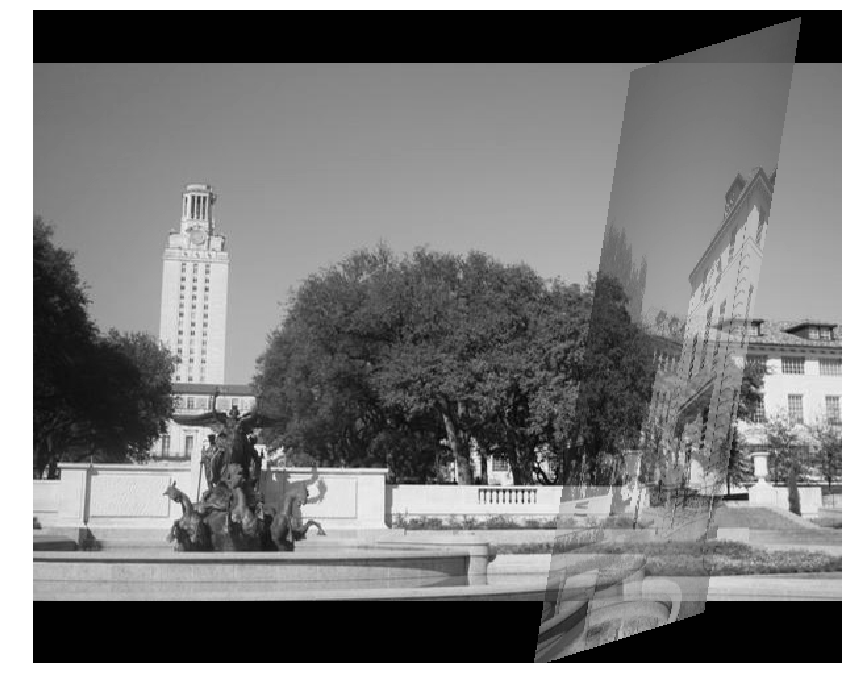
1 | merged = img1_warped + img2_warped |
2 | |
3 | # Track the overlap by adding the masks together |
4 | overlap = (img1_mask * 1.0 + # Multiply by 1.0 for bool -> float conversion |
5 | img2_mask) |
6 | |
7 | # Normalize through division by `overlap` - but ensure the minimum is 1 |
8 | normalized = merged / np.maximum(overlap, 1) |
9 | plt.imshow(normalized) |
10 | plt.axis('off') |
11 | plt.show() |
RANSAC
Rather than directly feeding all our keypoint matches into fit_affine_matrix function, we can instead use RANSAC (“RANdom SAmple Consensus”) to select only “inliers” to use to compute the transformation matrix.
The steps of RANSAC are:
- Select random set of matches
- Compute affine transformation matrix
- Find inliers using the given threshold
- Repeat and keep the largest set of inliers
- Re-compute least-squares estimate on all of the inliers
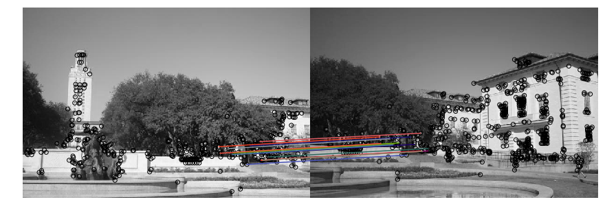
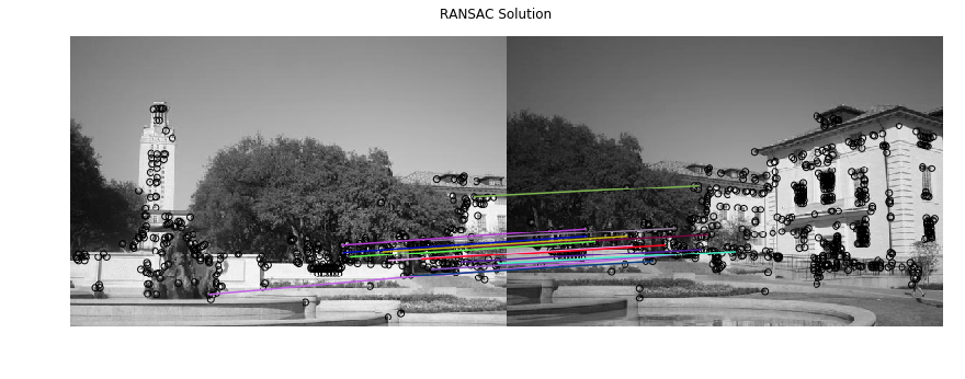
Implement ransac in panorama.py, run through the following code to get a panorama. You can see the difference from the result we get without RANSAC.
1 | from panorama import ransac |
2 | H, robust_matches = ransac(keypoints1, keypoints2, matches, threshold=1) |
3 | |
4 | # Visualize robust matches |
5 | fig, ax = plt.subplots(1, 1, figsize=(15, 12)) |
6 | plot_matches(ax, img1, img2, keypoints1, keypoints2, robust_matches) |
7 | plt.axis('off') |
8 | plt.show() |
9 | |
10 | plt.imshow(imread('solution_ransac.png')) |
11 | plt.axis('off') |
12 | plt.title('RANSAC Solution') |
13 | plt.show() |
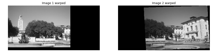
1 | output_shape, offset = get_output_space(img1, [img2], [H]) |
2 | |
3 | # Warp images into output sapce |
4 | img1_warped = warp_image(img1, np.eye(3), output_shape, offset) |
5 | img1_mask = (img1_warped != -1) # Mask == 1 inside the image |
6 | img1_warped[~img1_mask] = 0 # Return background values to 0 |
7 | |
8 | img2_warped = warp_image(img2, H, output_shape, offset) |
9 | img2_mask = (img2_warped != -1) # Mask == 1 inside the image |
10 | img2_warped[~img2_mask] = 0 # Return background values to 0 |
11 | |
12 | # Plot warped images |
13 | plt.subplot(1,2,1) |
14 | plt.imshow(img1_warped) |
15 | plt.title('Image 1 warped') |
16 | plt.axis('off') |
17 | |
18 | plt.subplot(1,2,2) |
19 | plt.imshow(img2_warped) |
20 | plt.title('Image 2 warped') |
21 | plt.axis('off') |
22 | |
23 | plt.show() |
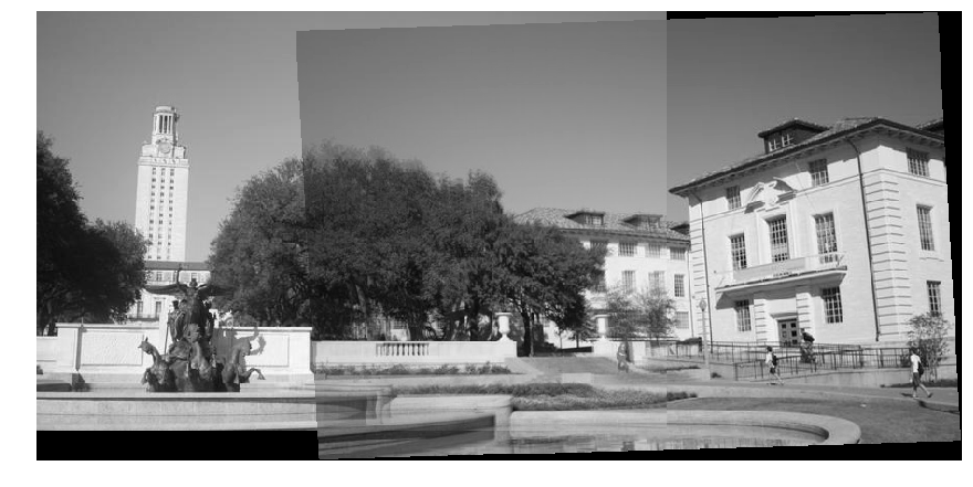
1 | merged = img1_warped + img2_warped |
2 | |
3 | # Track the overlap by adding the masks together |
4 | overlap = (img1_mask * 1.0 + # Multiply by 1.0 for bool -> float conversion |
5 | img2_mask) |
6 | |
7 | # Normalize through division by `overlap` - but ensure the minimum is 1 |
8 | normalized = merged / np.maximum(overlap, 1) |
9 | plt.imshow(normalized) |
10 | plt.axis('off') |
11 | plt.show() |
12 | |
13 | plt.imshow(imread('solution_ransac_panorama.png')) |
14 | plt.axis('off') |
15 | plt.title('RANSAC Panorama Solution') |
16 | plt.show() |

Histogram of Oriented Gradients (HOG)
In the above code, you are using the simple_descriptor, and in this section, you are going to implement a simplified version of HOG descriptor.
HOG stands for Histogram of Oriented Gradients. In HOG descriptor, the distribution ( histograms ) of directions of gradients ( oriented gradients ) are used as features. Gradients ( x and y derivatives ) of an image are useful because the magnitude of gradients is large around edges and corners ( regions of abrupt intensity changes ) and we know that edges and corners pack in a lot more information about object shape than flat regions.
The steps of HOG are:
- compute the gradient image in and
Use the sobel filter provided by skimage.filters- compute gradient histograms
Divide image into cells, and calculate histogram of gradient in each cell.- normalize across block
Normalize the histogram so that they- flattening block into a feature vector
Implement hog_descriptor in panorama.py, and run through the following code to get a panorama image.
关于HOG特征的算法流程,可以阅读此文
1 | from panorama import hog_descriptor |
2 | |
3 | img1 = imread('uttower1.jpg', as_grey=True) |
4 | img2 = imread('uttower2.jpg', as_grey=True) |
5 | |
6 | # Detect keypoints in both images |
7 | keypoints1 = corner_peaks(harris_corners(img1, window_size=3), |
8 | threshold_rel=0.05, |
9 | exclude_border=8) |
10 | keypoints2 = corner_peaks(harris_corners(img2, window_size=3), |
11 | threshold_rel=0.05, |
12 | exclude_border=8) |
1 | # Extract features from the corners |
2 | desc1 = describe_keypoints(img1, keypoints1, |
3 | desc_func=hog_descriptor, |
4 | patch_size=16) |
5 | desc2 = describe_keypoints(img2, keypoints2, |
6 | desc_func=hog_descriptor, |
7 | patch_size=16) |
8 | |
9 | # Match descriptors in image1 to those in image2 |
10 | matches = match_descriptors(desc1, desc2, 0.7) |
11 | |
12 | # Plot matches |
13 | fig, ax = plt.subplots(1, 1, figsize=(15, 12)) |
14 | ax.axis('off') |
15 | plot_matches(ax, img1, img2, keypoints1, keypoints2, matches) |
16 | plt.show() |
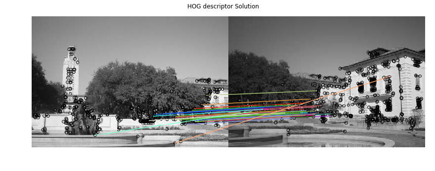
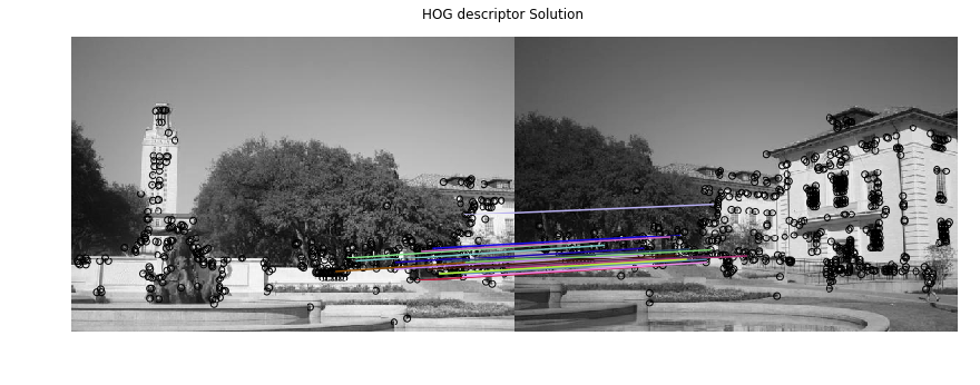
17 | plt.imshow(imread('solution_hog.png')) |
18 | plt.axis('off') |
19 | plt.title('HOG descriptor Solution') |
20 | plt.show() |
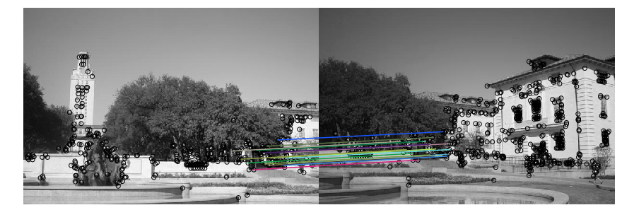
1 | from panorama import ransac |
2 | H, robust_matches = ransac(keypoints1, keypoints2, matches, threshold=1) |
3 | |
4 | # Plot matches |
5 | fig, ax = plt.subplots(1, 1, figsize=(15, 12)) |
6 | plot_matches(ax, img1, img2, keypoints1, keypoints2, robust_matches) |
7 | plt.axis('off') |
8 | plt.show() |
9 | |
10 | plt.imshow(imread('solution_hog_ransac.png')) |
11 | plt.axis('off') |
12 | plt.title('HOG descriptor Solution') |
13 | plt.show() |
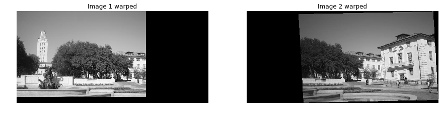
1 | output_shape, offset = get_output_space(img1, [img2], [H]) |
2 | |
3 | # Warp images into output sapce |
4 | img1_warped = warp_image(img1, np.eye(3), output_shape, offset) |
5 | img1_mask = (img1_warped != -1) # Mask == 1 inside the image |
6 | img1_warped[~img1_mask] = 0 # Return background values to 0 |
7 | |
8 | img2_warped = warp_image(img2, H, output_shape, offset) |
9 | img2_mask = (img2_warped != -1) # Mask == 1 inside the image |
10 | img2_warped[~img2_mask] = 0 # Return background values to 0 |
11 | |
12 | # Plot warped images |
13 | plt.subplot(1,2,1) |
14 | plt.imshow(img1_warped) |
15 | plt.title('Image 1 warped') |
16 | plt.axis('off') |
17 | |
18 | plt.subplot(1,2,2) |
19 | plt.imshow(img2_warped) |
20 | plt.title('Image 2 warped') |
21 | plt.axis('off') |
22 | |
23 | plt.show() |
1 | merged = img1_warped + img2_warped |
2 | |
3 | # merge之后重叠部分亮度上来了,需要通过归一化回复原来亮度 |
4 | # Track the overlap by adding the masks together |
5 | overlap = (img1_mask * 1.0 + # Multiply by 1.0 for bool -> float conversion |
6 | img2_mask) |
7 | |
8 | # Normalize through division by `overlap` - but ensure the minimum is 1 |
9 | normalized = merged / np.maximum(overlap, 1) |
10 | plt.imshow(normalized) |
11 | plt.axis('off') |
12 | plt.show() |
13 | |
14 | plt.imshow(imread('solution_hog_panorama.png')) |
15 | plt.axis('off') |
16 | plt.title('HOG Descriptor Panorama Solution') |
17 | plt.show() |

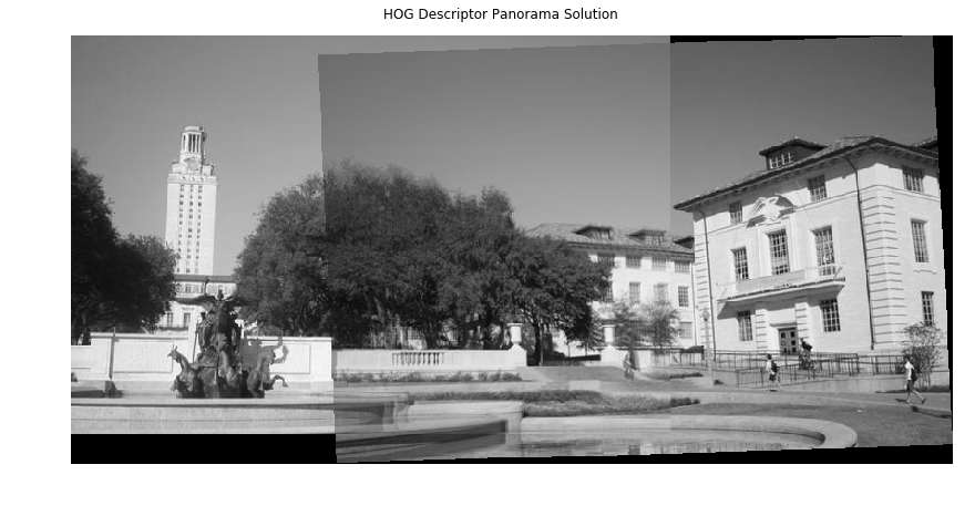
实现了HOG特征描述符之后,可以替代掉之前的归一化密度作为特征的匹配。效果不错。
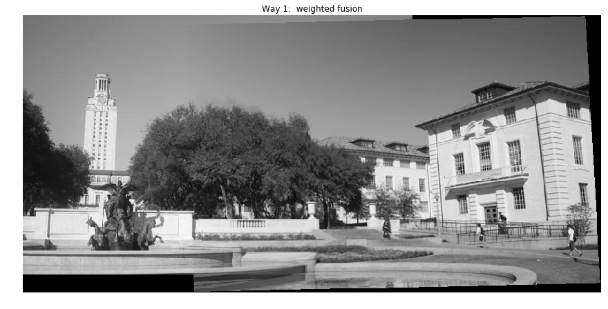
Extra Credit: Better Image Merging
You will notice the blurry region and unpleasant lines in the middle of the final panoramic image. In the cell below, come up with a better merging scheme to make the panorama look more natural. Be creative!
怎么消除拼接处的两条拼接痕迹呢?
加权融合
博客上的处理思路是加权融合,在重叠部分由前一幅图像慢慢过渡到第二幅图像,即将图像的重叠区域的像素值按一定的权值相加合成新的图像。
我的理解就是两块重叠的区域,从左向右每个像素由图1和图2融合,最开始图1的权重最大,图2的权重最小,向右融合过程中图1权重逐渐减小,图2权重逐渐增大。
融合的公式可以简单理解成:
而权重的值则与像素点在重叠区域的位置相关,可以定义成:
论文《Automatic Panoramic Image Stitching using Invariant Features》论文针对拼接步骤,提出了三点:
- 自动拼接校直 Automatic Panorama Straightening
校直是用BA做的相机参数的估计,用来解决拼接过程中的图像的旋转
- 增益补偿 Gain Compensation
增益补偿是用过使用最小二乘法计算每个拼接块的增益,用来均衡整幅图像中各个拼接块的亮度不均问题
- 多频带混合 Multi-Band Blending
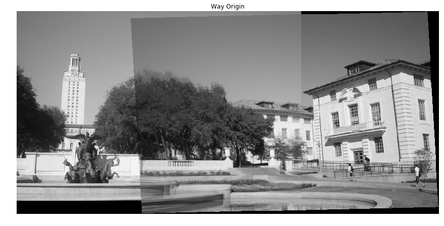
1 | # Modify the code below |
2 | |
3 | ### YOUR CODE HERE |
4 | |
5 | # # 拼接方法一:题目原有方法,两幅图叠加后在对重叠区域和非重叠区域做亮度调整。 |
6 | merged = img1_warped + img2_warped |
7 | overlap = (img1_mask * 1.0 + img2_mask) |
8 | output = merged / np.maximum(overlap, 1) |
9 | |
10 | plt.imshow(output) |
11 | plt.axis('off') |
12 | plt.title('Way Origin') |
13 | plt.show() |
14 | |
15 | # 拼接方法二:加权融合 |
16 | # 先把两幅图叠加在一起 |
17 | merged = img1_warped + img2_warped |
18 | # overlap = (img1_mask * 1.0 + img2_mask) |
19 | # output = merged / np.maximum(overlap, 1) |
20 | # 1. 找到重叠区域在warped图像中的左边界和右边界,可以根据已知的mask图像进行判断 |
21 | # 1.1 重叠区域左边界就是img2_mask中第一个不全为零的列 |
22 | for col in range(img2_warped.shape[1]): |
23 | if not np.all(img2_mask[:, col] == False): |
24 | break |
25 | regionLeft = col |
26 | # 1.2 重叠区域右边界就是img1_mask中有值区域的右边,其实就是img1的宽所在的列 |
27 | regionRight = img1.shape[1] |
28 | # 1.3 区域宽度 |
29 | regionWidth = regionRight - regionLeft + 1 |
30 | |
31 | # 2. 遍历区域内像素点进行融合 |
32 | for col in range(regionLeft, regionRight+1): |
33 | for row in range(img2_warped.shape[0]): |
34 | # 2.1 计算α |
35 | alpha = (col - regionLeft) / (regionWidth) |
36 | alpha = 1 - alpha |
37 | # 2.2 处理区域内的重叠点 |
38 | if img1_mask[row,col] and img2_mask[row,col]: |
39 | merged[row,col] = alpha * img1_warped[row,col] + (1 - alpha) * img2_warped[row,col] |
40 | |
41 | output = merged |
42 | |
43 | plt.imshow(output) |
44 | plt.axis('off') |
45 | plt.title('Way 1: weighted fusion') |
46 | plt.show() |
47 | ### END YOUR CODE |
OpenPano
Github上宇哥开源的拼接库OpenPano
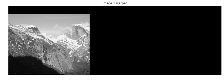
Extra Credit: Stitching Multiple Images
Work in the cell below to complete the code to stitch an ordered chain of images.
Given a sequence of m images , take every neighboring pair of images and compute the transformation matrix which converts points from the coordinate frame of to the frame of . Then, select a reference image , which is in the middle of the chain. We want our final panorama image to be in the coordinate frame of . So, for each that is not the reference image, we need a transformation matrix that will convert points in frame to frame .
-Hint:
- If you are confused, you may want to review the Linear Algebra slides on how to combine the effects of multiple transformation matrices.
- The inverse of transformation matrix has the reverse effect. Please use numpy.linalg.inv function whenever you want to compute matrix inverse.
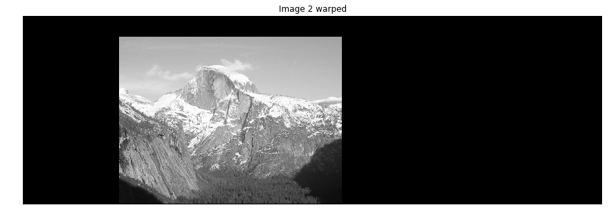
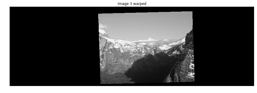
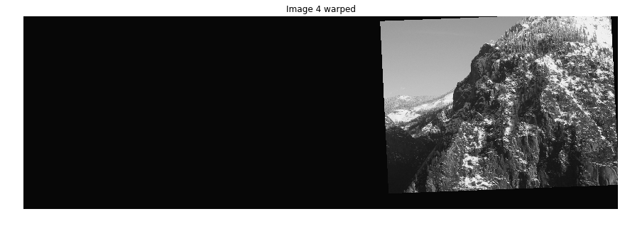
1 | img1 = imread('yosemite1.jpg', as_grey=True) |
2 | img2 = imread('yosemite2.jpg', as_grey=True) |
3 | img3 = imread('yosemite3.jpg', as_grey=True) |
4 | img4 = imread('yosemite4.jpg', as_grey=True) |
5 | |
6 | # Detect keypoints in each image |
7 | keypoints1 = corner_peaks(harris_corners(img1, window_size=3), |
8 | threshold_rel=0.05, |
9 | exclude_border=8) |
10 | keypoints2 = corner_peaks(harris_corners(img2, window_size=3), |
11 | threshold_rel=0.05, |
12 | exclude_border=8) |
13 | keypoints3 = corner_peaks(harris_corners(img3, window_size=3), |
14 | threshold_rel=0.05, |
15 | exclude_border=8) |
16 | keypoints4 = corner_peaks(harris_corners(img4, window_size=3), |
17 | threshold_rel=0.05, |
18 | exclude_border=8) |
19 | |
20 | # Describe keypoints |
21 | desc1 = describe_keypoints(img1, keypoints1, |
22 | desc_func=simple_descriptor, |
23 | patch_size=patch_size) |
24 | desc2 = describe_keypoints(img2, keypoints2, |
25 | desc_func=simple_descriptor, |
26 | patch_size=patch_size) |
27 | desc3 = describe_keypoints(img3, keypoints3, |
28 | desc_func=simple_descriptor, |
29 | patch_size=patch_size) |
30 | desc4 = describe_keypoints(img4, keypoints4, |
31 | desc_func=simple_descriptor, |
32 | patch_size=patch_size) |
33 | |
34 | # Match keypoints in neighboring images |
35 | matches12 = match_descriptors(desc1, desc2, 0.7) |
36 | matches23 = match_descriptors(desc2, desc3, 0.7) |
37 | matches34 = match_descriptors(desc3, desc4, 0.7) |
38 | |
39 | ### YOUR CODE HERE |
40 | # RANSAC 估计 仿射变换矩阵 |
41 | H12, robust_matches12 = ransac(keypoints1, keypoints2, matches12, threshold=1) |
42 | H23, robust_matches23 = ransac(keypoints2, keypoints3, matches23, threshold=1) |
43 | H34, robust_matches34 = ransac(keypoints3, keypoints4, matches34, threshold=1) |
44 | |
45 | # 生成outspace大背景 |
46 | # 注意utils.py中的get_output_space用法,参数2:imgs与参数3:transforms要对应 |
47 | # 注意选取referImg 参考图像,这里选择图2 |
48 | output_shape, offset = get_output_space(img2, [img1, img3, img4], [np.linalg.inv(H12), H23, np.dot(H23,H34)]) |
49 | |
50 | # 将图像放入大背景中 |
51 | # Warp images into output sapce |
52 | img1_warped = warp_image(img1, np.linalg.inv(H12), output_shape, offset) |
53 | img1_mask = (img1_warped != -1) # Mask == 1 inside the image |
54 | img1_warped[~img1_mask] = 0 # Return background values to 0 |
55 | |
56 | img2_warped = warp_image(img2, np.eye(3), output_shape, offset) |
57 | img2_mask = (img2_warped != -1) # Mask == 1 inside the image |
58 | img2_warped[~img2_mask] = 0 # Return background values to 0 |
59 | |
60 | img3_warped = warp_image(img3, H23, output_shape, offset) |
61 | img3_mask = (img3_warped != -1) # Mask == 1 inside the image |
62 | img3_warped[~img3_mask] = 0 # Return background values to 0 |
63 | |
64 | img4_warped = warp_image(img4, np.dot(H23,H34), output_shape, offset) |
65 | img4_mask = (img4_warped != -1) # Mask == 1 inside the image |
66 | img4_warped[~img4_mask] = 0 # Return background values to 0 |
67 | |
68 | |
69 | plt.imshow(img1_warped) |
70 | plt.axis('off') |
71 | plt.title('Image 1 warped') |
72 | plt.show() |
73 | |
74 | plt.imshow(img2_warped) |
75 | plt.axis('off') |
76 | plt.title('Image 2 warped') |
77 | plt.show() |
78 | |
79 | plt.imshow(img3_warped) |
80 | plt.axis('off') |
81 | plt.title('Image 3 warped') |
82 | plt.show() |
83 | |
84 | plt.imshow(img4_warped) |
85 | plt.axis('off') |
86 | plt.title('Image 4 warped') |
87 | plt.show() |
88 | |
89 | ### END YOUR CODE |
1 | # 进行拼接,拼接方式一 |
2 | merged = img1_warped + img2_warped + img3_warped + img4_warped |
3 | |
4 | # Track the overlap by adding the masks together |
5 | overlap = (img2_mask * 1.0 + # Multiply by 1.0 for bool -> float conversion |
6 | img1_mask + img3_mask + img4_mask) |
7 | |
8 | # Normalize through division by `overlap` - but ensure the minimum is 1 |
9 | normalized = merged / np.maximum(overlap, 1) |
10 | |
11 | plt.imshow(normalized) |
12 | plt.show() |
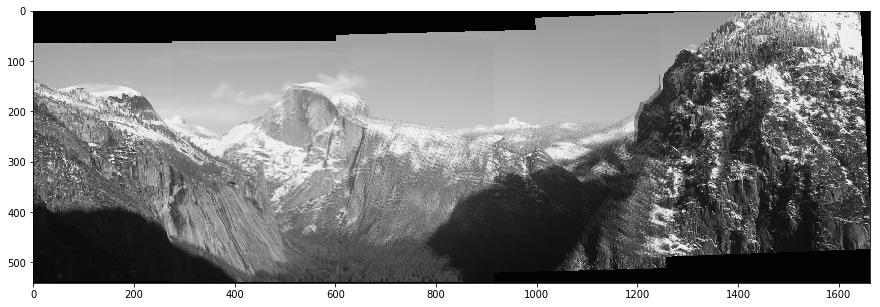
多幅图的拼接就可以看出来简单方式的问题了:
- 拼接痕迹的存在,可以使用加权平均,
- 各个拼接块亮度不均匀,需要做增益补偿,
- 存在未知的图像的旋转,可能是由于拍摄时相机发生了位姿的变动,需要做优化处理(校直),
- 重叠部分的拼接并不能直接实现所有像素的对应叠加,可以看出来存在模糊的情况,可以使用多频带混合的方式去做处理。
Resizing-SeamCarving
复现Seam Carving(接缝拼接)算法,实现基于内容感知的图像智能缩放,并且实现图像中目标的移除,了解图像能量图、动态编程。
@Reference
CS131: Computer Vision Foundations and Applications
The material presented here is inspired from:
The whole seam carving process was covered in lecture 8, please refer to the slides for more details to the different concepts introduced here.
这份作业的主题是实现SeamCarving(接缝裁剪)的算法,即基于图像内容感知的图像缩放算法。
- 实现图像裁剪
- 实现图像扩大
- 其他实验
也可以参考这篇专栏讲了如何用Python实现Seam carving算法,原理讲解的挺清楚的。
如何用Python实现神奇切图算法Seam Carving ?
Sean Carving 的基本思路
- 计算图像能量图
- 寻找最小能量线
- 移除得到的最小能量线,让图片的宽度缩小一个像素
Seam carving is an algorithm for content-aware image resizing.
To understand all the concepts in this homework, make sure to read again the slides from lecture 8
http://vision.stanford.edu/teaching/cs131_fall1718/files/08_seam_carving.pdf
1 | from skimage import io, util |
2 | |
3 | # Load image |
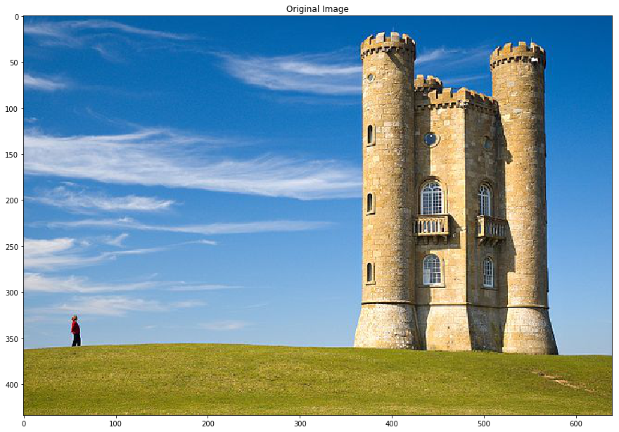
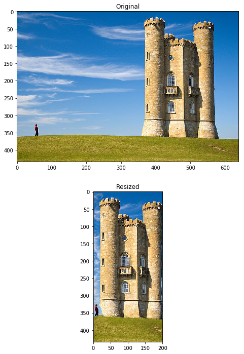
4 | img = io.imread('imgs/broadway_tower.jpg') |
5 | img = util.img_as_float(img) |
6 | |
7 | plt.title('Original Image') |
8 | plt.imshow(img) |
9 | plt.show() |
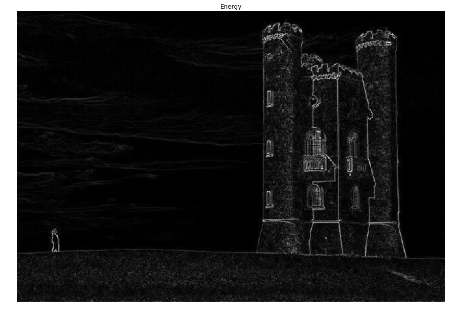
Energy function
We will now implemented the energy_function to compute the energy of the image.
The energy at each pixel is the sum of:
- absolute value of the gradient in the direction
- absolute value of the gradient in the direction
The function should take around 0.01 to 0.1 seconds to compute.
图像能量图此处定义为图像每个像素的两方向梯度幅值之和,当然能量也可以是别的定义方式:梯度幅度、熵图、显著图等等。计算梯度要注意转换为灰度图再进行。
1 | from seam_carving import energy_function |
2 | |
3 | test_img = np.array([[1.0, 2.0, 1.5], |
4 | [3.0, 1.0, 2.0], |
5 | [4.0, 0.5, 3.0]]) |
6 | test_img = np.stack([test_img] * 3, axis=2) |
7 | assert test_img.shape == (3, 3, 3) |
8 | |
9 | # Compute energy function |
10 | test_energy = energy_function(test_img) |
11 | |
12 | solution_energy = np.array([[3.0, 1.25, 1.0], |
13 | [3.5, 1.25, 1.75], |
14 | [4.5, 1.0, 3.5]]) |
15 | |
16 | print("Image (channel 0):") |
17 | print(test_img[:, :, 0]) |
18 | |
19 | print("Energy:") |
20 | print(test_energy) |
21 | print("Solution energy:") |
22 | print(solution_energy) |
23 | |
24 | assert np.allclose(test_energy, solution_energy) |
1 | # Compute energy function |
2 | start = time() |
3 | energy = energy_function(img) |
4 | end = time() |
5 | |
6 | print("Computing energy function: %f seconds." % (end - start)) |
7 | |
8 | plt.title('Energy') |
9 | plt.axis('off') |
10 | plt.imshow(energy) |
11 | plt.show() |
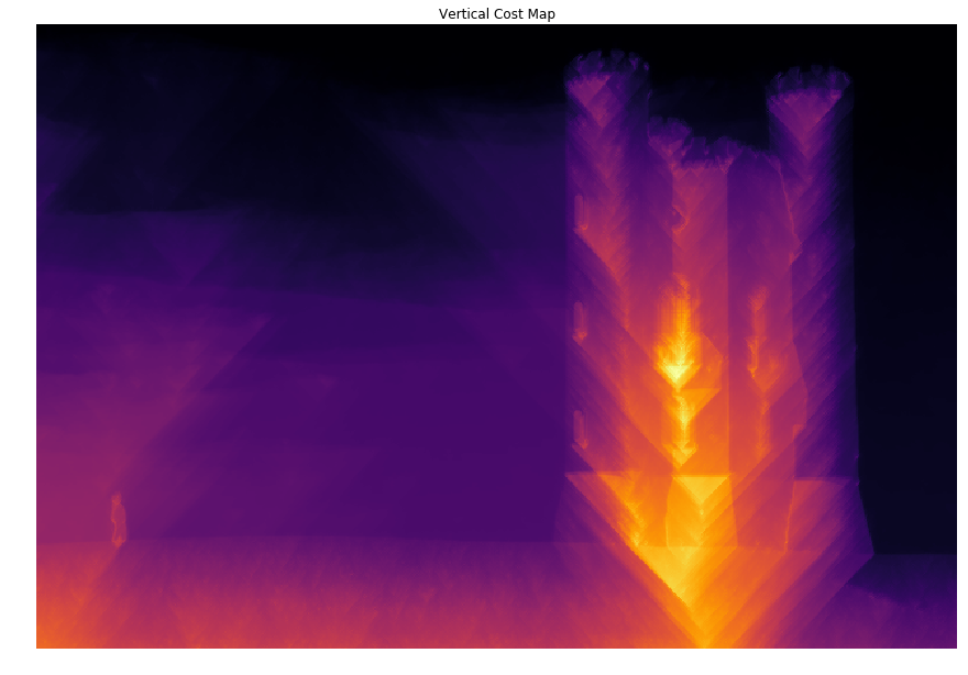
Compute cost
Now implement the function compute_cost.
Starting from the energy map, we’ll go from the first row of the image to the bottom and compute the minimal cost at each pixel.
We’ll use dynamic programming to compute the cost line by line starting from the first row.
The function should take around 0.05 seconds to complete.
此处要求使用动态规划计算整幅图的cost图,用于第三步寻找最小能量线。
此处动态规划的意思是从图像的最上面一行开始,计算能量的最小累加路线,cost图中每一行的每个像素从它八相邻的上一行的三个像素中取最小cost值的元素进行累加。
直到累加到最后一行,同时在计算过程中保留每个像素的累加路径,即像素的cost值是从上一行哪一个元素相加得到的(用-1,0,1表示上左,上中,上右)。
题目中要求只用一个循环实现,则需要用向量化的形式进行计算。
1 | from seam_carving import compute_cost |
2 | |
3 | # Let's first test with a small example |
4 | |
5 | test_energy = np.array([[1.0, 2.0, 1.5], |
6 | [3.0, 1.0, 2.0], |
7 | [4.0, 0.5, 3.0]]) |
8 | |
9 | solution_cost = np.array([[1.0, 2.0, 1.5], |
10 | [4.0, 2.0, 3.5], |
11 | [6.0, 2.5, 5.0]]) |
12 | |
13 | solution_paths = np.array([[ 0, 0, 0], |
14 | [ 0, -1, 0], |
15 | [ 1, 0, -1]]) |
16 | |
17 | # Vertical Cost Map |
18 | vcost, vpaths = compute_cost(_, test_energy, axis=1) # don't need the first argument for compute_cost |
19 | |
20 | print("Energy:") |
21 | print(test_energy) |
22 | |
23 | print("Cost:") |
24 | print(vcost) |
25 | print("Solution cost:") |
26 | print(solution_cost) |
27 | |
28 | print("Paths:") |
29 | print(vpaths) |
30 | print("Solution paths:") |
31 | print(solution_paths) |
1 | # Vertical Cost Map |
2 | start = time() |
3 | vcost, _ = compute_cost(_, energy, axis=1) # don't need the first argument for compute_cost |
4 | end = time() |
5 | |
6 | print("Computing vertical cost map: %f seconds." % (end - start)) |
7 | |
8 | plt.title('Vertical Cost Map') |
9 | plt.axis('off') |
10 | plt.imshow(vcost, cmap='inferno') |
11 | plt.show() |
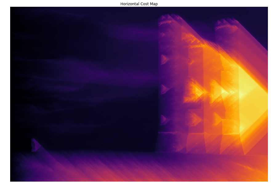
1 | # Horizontal Cost Map |
2 | start = time() |
3 | hcost, _ = compute_cost(_, energy, axis=0) |
4 | end = time() |
5 | |
6 | print("Computing horizontal cost map: %f seconds." % (end - start)) |
7 | |
8 | plt.title('Horizontal Cost Map') |
9 | plt.axis('off') |
10 | plt.imshow(hcost, cmap='inferno') |
11 | plt.show() |
Finding optimal seams
Using the cost maps we found above, we can determine the seam with the lowest energy in the image.
We can then remove this optimal seam, and repeat the process until we obtain a desired width.
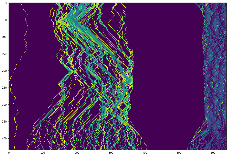
由于上面计算能量cost图时,已经保存了每个像素点的叠加路径,因此可以在最后一行找到最小的cost,并从该点开始,向上溯源,找到一条最佳的接缝,即最小的能量线。
Backtrack seam
Implement function backtrack_seam
1 | from seam_carving import backtrack_seam |
2 | |
3 | # Let's first test with a small example |
4 | cost = np.array([[1.0, 2.0, 1.5], |
5 | [4.0, 2.0, 3.5], |
6 | [6.0, 2.5, 5.0]]) |
7 | |
8 | paths = np.array([[ 0, 0, 0], |
9 | [ 0, -1, 0], |
10 | [ 1, 0, -1]]) |
11 | |
12 | |
13 | # Vertical Backtracking |
14 | |
15 | end = np.argmin(cost[-1]) |
16 | seam_energy = cost[-1, end] |
17 | seam = backtrack_seam(vpaths, end) |
18 | |
19 | print('Seam Energy:', seam_energy) |
20 | print('Seam:', seam) |
21 | |
22 | assert seam_energy == 2.5 |
23 | assert np.allclose(seam, [0, 1, 1]) |
1 | vcost, vpaths = compute_cost(img, energy) |
2 | |
3 | # Vertical Backtracking |
4 | start = time() |
5 | end = np.argmin(vcost[-1]) |
6 | seam_energy = vcost[-1, end] |
7 | seam = backtrack_seam(vpaths, end) |
8 | end = time() |
9 | |
10 | print("Backtracking optimal seam: %f seconds." % (end - start)) |
11 | print('Seam Energy:', seam_energy) |
12 | |
13 | # Visualize seam |
14 | vseam = np.copy(img) |
15 | for row in range(vseam.shape[0]): |
16 | vseam[row, seam[row], :] = np.array([1.0, 0, 0]) |
17 | |
18 | plt.title('Vertical Seam') |
19 | plt.axis('off') |
20 | plt.imshow(vseam) |
21 | plt.show() |
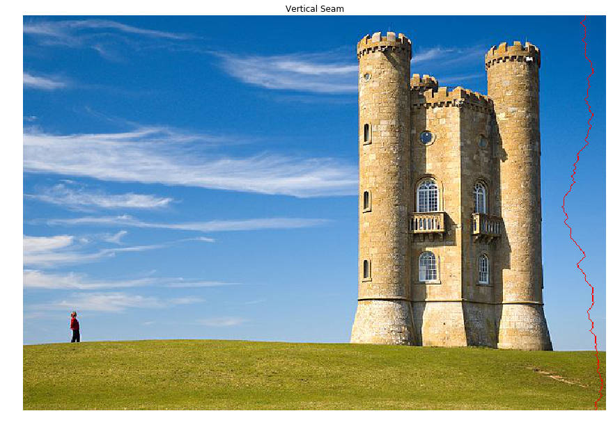
到此,就实现了一条接缝的查找,接下来移除它就可以实现一个像素宽度的缩小。
In the image above, the optimal vertical seam (minimal cost) goes through the portion of sky without any cloud, which yields the lowest energy.
Reduce
We can now use the function backtrack and remove_seam iteratively to reduce the size of the image through seam carving.
Each reduce can take around 10 seconds to compute, depending on your implementation.
If it’s too long, try to vectorize your code in compute_cost to only use one loop.
1 | from seam_carving import reduce |
2 | |
3 | # Let's first test with a small example |
4 | test_img = np.arange(9, dtype=np.float64).reshape((3, 3)) |
5 | test_img = np.stack([test_img, test_img, test_img], axis=2) |
6 | assert test_img.shape == (3, 3, 3) |
7 | |
8 | cost = np.array([[1.0, 2.0, 1.5], |
9 | [4.0, 2.0, 3.5], |
10 | [6.0, 2.5, 5.0]]) |
11 | |
12 | paths = np.array([[ 0, 0, 0], |
13 | [ 0, -1, 0], |
14 | [ 1, 0, -1]]) |
15 | |
16 | # Reduce image width |
17 | W_new = 2 |
18 | |
19 | # We force the cost and paths to our values |
20 | out = reduce(test_img, W_new, cfunc=lambda x, y: (cost, paths)) |
21 | |
22 | print("Original image (channel 0):") |
23 | print(test_img[:, :, 0]) |
24 | print("Reduced image (channel 0): we see that seam [0, 4, 7] is removed") |
25 | print(out[:, :, 0]) |
26 | |
27 | assert np.allclose(out[:, :, 0], np.array([[1, 2], [3, 5], [6, 8]])) |
1 | # Reduce image width |
2 | H, W, _ = img.shape |
3 | W_new = 400 |
4 | |
5 | start = time() |
6 | out = reduce(img, W_new) |
7 | end = time() |
8 | |
9 | print("Reducing width from %d to %d: %f seconds." % (W, W_new, end - start)) |
10 | |
11 | plt.subplot(2, 1, 1) |
12 | plt.title('Original') |
13 | plt.imshow(img) |
14 | |
15 | plt.subplot(2, 1, 2) |
16 | plt.title('Resized') |
17 | plt.imshow(out) |
18 | |
19 | plt.show() |
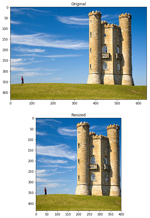
裁剪部分我是按照每一行删除一个元素的方式去实现的。
能够达到题目要求的10s左右的时间要求。
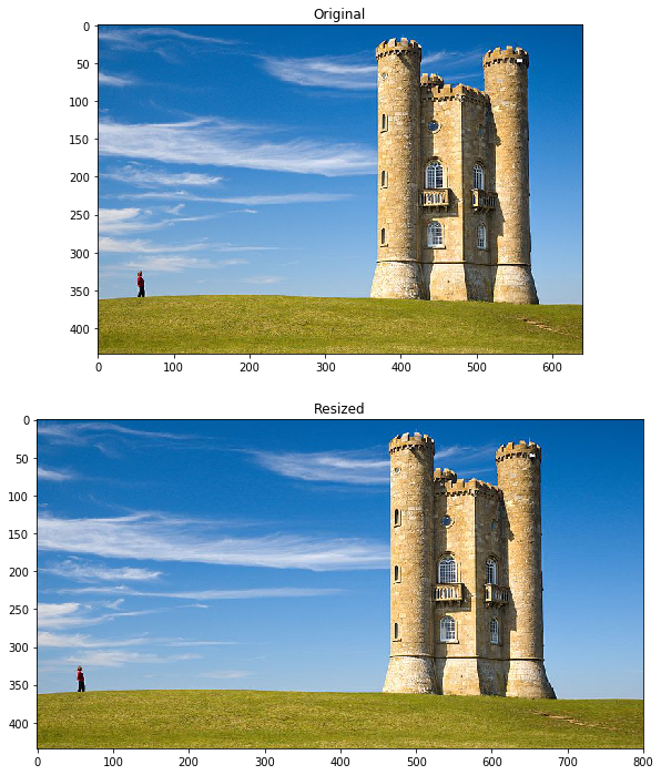
We observe that resizing from width 640 to width 400 conserves almost all the important part of the image (the person and the castle), where a standard resizing would have compressed everything.
All the vertical seams removed avoid the person and the castle.
程序同样可以缩减高度,程序中对于另一个维度的裁剪做了判断,
只需要seam carving流程走之前旋转图像,走完流程之后再将裁剪宽度的图像旋转回来就成了裁剪高度了。
1 | # Reduce image height |
2 | H, W, _ = img.shape |
3 | H_new = 300 |
4 | |
5 | start = time() |
6 | out = reduce(img, H_new, axis=0) |
7 | end = time() |
8 | |
9 | print("Reducing height from %d to %d: %f seconds." % (H, H_new, end - start)) |
10 | |
11 | plt.subplot(1, 2, 1) |
12 | plt.title('Original') |
13 | plt.imshow(img) |
14 | |
15 | plt.subplot(1, 2, 2) |
16 | plt.title('Resized') |
17 | plt.imshow(out) |
18 | |
19 | plt.show() |
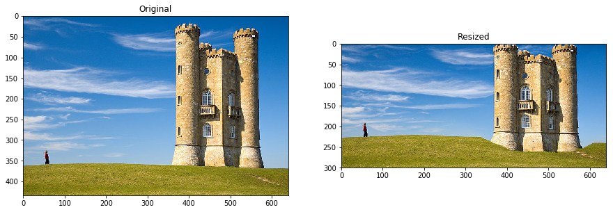
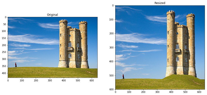
For reducing the height, we observe that the result does not look as nice.
The issue here is that the castle is on all the height of the image, so most horizontal seams will go through it.
Interestingly, we observe that most of the grass is not removed. This is because the grass has small variation between neighboring pixels (in a kind of noisy pattern) that make it high energy.
The seams removed go through the sky on the left, go under the castle to remove some grass and then back up in the low energy blue sky.
虽然实现了高度的裁剪,但是图像看起来怪怪的,这是可以从图像上做分析的。
城堡明显具有很强的能量,详见第一步能量图计算,因此裁剪高度时,每一条最小能量线都会越过它。
草坪看起来其实跟噪声一样,每个像素点与相邻像素都有或大或小的差异,因此梯度也是较大的,因此能量也较高,不会首先裁剪草坪而是更平滑的蓝天,
而城堡下面的草坪凹陷是因为城堡上方的蓝天已被裁剪光了,最小能量线无法从上方穿过时才从城堡下方的草坪开始裁剪的。
Image Enlarging
Enlarge naive
We now want to tackle the reverse problem of enlarging an image.
One naive way to approach the problem would be to duplicate the optimal seam iteratively until we reach the desired size.
图像扩大的一种方式是直接在最小能量线的地方复制它。
在enlarge_naive函数中实现它。
1 | from seam_carving import enlarge_naive |
2 | |
3 | # Let's first test with a small example |
4 | test_img = np.arange(9, dtype=np.float64).reshape((3, 3)) |
5 | test_img = np.stack([test_img, test_img, test_img], axis=2) |
6 | assert test_img.shape == (3, 3, 3) |
7 | |
8 | cost = np.array([[1.0, 2.0, 1.5], |
9 | [4.0, 2.0, 3.5], |
10 | [6.0, 2.5, 5.0]]) |
11 | |
12 | paths = np.array([[ 0, 0, 0], |
13 | [ 0, -1, 0], |
14 | [ 1, 0, -1]]) |
15 | |
16 | # Increase image width |
17 | W_new = 4 |
18 | |
19 | # We force the cost and paths to our values |
20 | out = enlarge_naive(test_img, W_new, cfunc=lambda x, y: (cost, paths)) |
21 | |
22 | print("Original image (channel 0):") |
23 | print(test_img[:, :, 0]) |
24 | print("Enlarged image (channel 0): we see that seam [0, 4, 7] is duplicated") |
25 | print(out[:, :, 0]) |
26 | |
27 | assert np.allclose(out[:, :, 0], np.array([[0, 0, 1, 2], [3, 4, 4, 5], [6, 7, 7, 8]])) |
1 | W_new = 800 |
2 | |
3 | # This is a naive implementation of image enlarging |
4 | # which iteratively computes energy function, finds optimal seam |
5 | # and duplicates it. |
6 | # This process will a stretching artifact by choosing the same seam |
7 | start = time() |
8 | enlarged = enlarge_naive(img, W_new) |
9 | end = time() |
10 | |
11 | # Can take around 20 seconds |
12 | print("Enlarging(naive) height from %d to %d: %f seconds." \ |
13 | % (W, W_new, end - start)) |
14 | |
15 | plt.imshow(enlarged) |
16 | plt.show() |
The issue with enlarge_naive is that the same seam will be selected again and again, so this low energy seam will be the only to be duplicated.
Another way to get k different seams is to apply the process we used in function reduce, and keeping track of the seams we delete progressively.
The function find_seams(image, k) will find the top k seams for removal iteratively.
The inner workings of the function are a bit tricky so we’ve implemented it for you, but you should go into the code and understand how it works.
This should also help you for the implementation of enlarge.
作业已经帮忙实现了:查找k条不同的接缝,这样就可以根据k条接缝来轮流进行删除了。
1 | from seam_carving import find_seams |
2 | |
3 | # Alternatively, find k seams for removal and duplicate them. |
4 | start = time() |
5 | seams = find_seams(img, W_new - W) |
6 | end = time() |
7 | |
8 | # Can take around 10 seconds |
9 | print("Finding %d seams: %f seconds." % (W_new - W, end - start)) |
10 | |
11 | plt.imshow(seams, cmap='viridis') |
12 | plt.show() |
不同的颜色是因为按照排序,给每条路线的标记的值不同。
Enlarge
We can see that all the seams found are different, and they avoid the castle and the person.
One issue we can mention is that we cannot enlarge more than we can reduce. Because of our process, the maximum enlargement is the width of the image W because we first need to find W different seams in the image.
One effect we can see on this image is that the blue sky at the right of the castle can only be enlarged x2. The concentration of seams in this area is very strong.
We can also note that the seams at the right of the castle have a blue color, which means they have low value and were removed in priority in the seam selection process.
值得注意的是,对于图像能放大的像素宽度肯定不会超过图像能缩减的像素宽度,毕竟最小能量线就只有那么多条。
实现enlarge函数。
1 | from seam_carving import enlarge |
2 | |
3 | # Let's first test with a small example |
4 | test_img = np.array([[0.0, 1.0, 3.0], |
5 | [0.0, 1.0, 3.0], |
6 | [0.0, 1.0, 3.0]]) |
7 | #test_img = np.arange(9, dtype=np.float64).reshape((3, 3)) |
8 | test_img = np.stack([test_img, test_img, test_img], axis=2) |
9 | assert test_img.shape == (3, 3, 3) |
10 | |
11 | # Increase image width |
12 | W_new = 5 |
13 | |
14 | out_naive = enlarge_naive(test_img, W_new) |
15 | out = enlarge(test_img, W_new) |
16 | |
17 | print("Original image (channel 0):") |
18 | print(test_img[:, :, 0]) |
19 | print("Enlarged naive image (channel 0): first seam is duplicated twice.") |
20 | print(out_naive[:, :, 0]) |
21 | print("Enlarged image (channel 0): first and second seam are each duplicated once.") |
22 | print(out[:, :, 0]) |
23 | |
24 | assert np.allclose(out[:, :, 0], np.array([[0, 0, 1, 1, 3], [0, 0, 1, 1, 3], [0, 0, 1, 1, 3]])) |
1 | W_new = 800 |
2 | |
3 | start = time() |
4 | out = enlarge(img, W_new) |
5 | end = time() |
6 | |
7 | # Can take around 20 seconds |
8 | print("Enlarging width from %d to %d: %f seconds." \ |
9 | % (W, W_new, end - start)) |
10 | |
11 | plt.subplot(2, 1, 1) |
12 | plt.title('Original') |
13 | plt.imshow(img) |
14 | |
15 | plt.subplot(2, 1, 2) |
16 | plt.title('Resized') |
17 | plt.imshow(out) |
18 | |
19 | plt.show() |
1 | # Map of the seams for horizontal seams. |
2 | start = time() |
3 | seams = find_seams(img, W_new - W, axis=0) |
4 | end = time() |
5 | |
6 | # Can take around 15 seconds |
7 | print("Finding %d seams: %f seconds." % (W_new - W, end - start)) |
8 | |
9 | plt.imshow(seams, cmap='viridis') |
10 | plt.show() |
1 | H_new = 600 |
2 | |
3 | start = time() |
4 | out = enlarge(img, H_new, axis=0) |
5 | end = time() |
6 | |
7 | # Can take around 20 seconds |
8 | print("Enlarging height from %d to %d: %f seconds." \ |
9 | % (H, H_new, end - start)) |
10 | |
11 | plt.subplot(1, 2, 1) |
12 | plt.title('Original') |
13 | plt.imshow(img) |
14 | |
15 | plt.subplot(1, 2, 2) |
16 | plt.title('Resized') |
17 | plt.imshow(out) |
18 | |
19 | plt.show() |
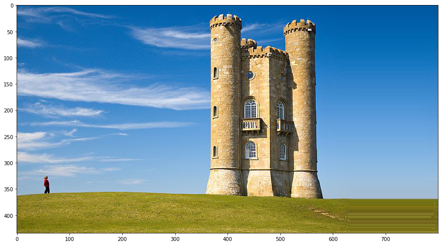
As you can see in the example above, the sky above the castle has doubled in size, the grass below has doubled in size but we still can’t reach a height of 600.
The algorithm then needs to enlarge the castle itself, while trying to avoid enlarging the windows for instance.
Other experiments on the image
Feel free to experiment more on this image, try different sizes to enlarge or reduce, or check what seams are chosen…
Reducing by a 2x factor often leads to weird patterns.
Enlarging by more than 2x is impossible since we only duplicate seams. One solution is to enlarge in mutliple steps (enlarge x1.4, enlarge again x1.4…)
放大两倍或者缩小二分之一图像会变得很奇怪。
这里提出一个方式就是进行多次Resize步骤,每次x1.4倍,x1.4倍这样的方式来放大,缩小同理。
1 | # Reduce image width |
2 | H, W, _ = img.shape |
3 | W_new = 200 |
4 | |
5 | start = time() |
6 | out = reduce(img, W_new) |
7 | end = time() |
8 | |
9 | print("Reducing width from %d to %d: %f seconds." % (W, W_new, end - start)) |
10 | |
11 | plt.subplot(2, 1, 1) |
12 | plt.title('Original') |
13 | plt.imshow(img) |
14 | |
15 | plt.subplot(2, 1, 2) |
16 | plt.title('Resized') |
17 | plt.imshow(out) |
18 | |
19 | plt.show() |
Faster reduce (extra credit 0.5%)
Implement a faster version of reduce called reduce_fast in the file seam_carving.py.
We will have a leaderboard on gradescope with the performance of students.
The autograder tests will check that the outputs match, and run the reduce_fast function on a set of images with varying shapes (say between 200 and 800).
怎么能实现更快地裁剪呢?
题目的提示是:do we really need to compute the whole cost map again at each iteration?
分析了一下reduce的过程,的确有一块是可以改进的。
1 | while out.shape[1] > size: |
2 | energy = efunc(out) |
3 | cost, paths = cfunc(out, energy) |
4 | end = np.argmin(cost[-1]) |
5 | seam = backtrack_seam(paths, end) |
6 | out = remove_seam(out, seam) |
就是计算energy能量图这一步,因为能量图的计算其实就是梯度的计算。
如果一个区域内的图像像素不变动的话,那这个区域内的梯度应该也不会放生改变,基于这一点,可以对计算能量图的步骤进行改进。
只需要对上一次optical seam最小能量线覆盖宽度内的区域进行梯度的重新更新,两侧区域的能量值不需要变动。
比如接缝最左边为left,则left-1处像素不变,梯度改变,left-2处及之前像素不变梯度不变。
比如接缝最右边为right,则right+1处像素不变,梯度改变,left+2处及之后像素不变梯度不变。
然后考虑特殊情况。
1 | from seam_carving import reduce_fast |
2 | |
3 | # Reduce image width |
4 | H, W, _ = img.shape |
5 | W_new = 400 |
6 | |
7 | start = time() |
8 | out = reduce(img, W_new) |
9 | end = time() |
10 | |
11 | print("Normal reduce width from %d to %d: %f seconds." % (W, W_new, end - start)) |
12 | |
13 | start = time() |
14 | out_fast = reduce_fast(img, W_new) |
15 | end = time() |
16 | |
17 | print("Faster reduce width from %d to %d: %f seconds." % (W, W_new, end - start)) |
18 | |
19 | assert np.allclose(out, out_fast), "Outputs don't match." |
20 | |
21 | |
22 | plt.subplot(3, 1, 1) |
23 | plt.title('Original') |
24 | plt.imshow(img) |
25 | |
26 | plt.subplot(3, 1, 2) |
27 | plt.title('Resized') |
28 | plt.imshow(out) |
29 | |
30 | plt.subplot(3, 1, 3) |
31 | plt.title('Faster resized') |
32 | plt.imshow(out) |
33 | |
34 | plt.show() |
Reducing and enlarging on another image
Also check these outputs with another image.
1 | # Load image |
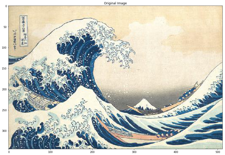
2 | img2 = io.imread('imgs/wave.jpg') |
3 | img2 = util.img_as_float(img2) |
4 | |
5 | plt.title('Original Image') |
6 | plt.imshow(img2) |
7 | plt.show() |
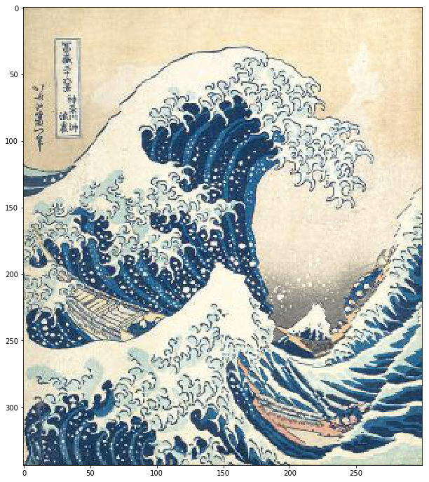
1 | out = reduce(img2, 300) |
2 | plt.imshow(out) |
3 | plt.show() |
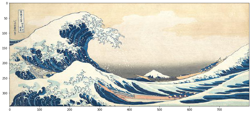
1 | out = enlarge(img2, 800) |
2 | plt.imshow(out) |
3 | plt.show() |
Forward Energy
Forward energy is a solution to some artifacts that appear when images have curves for instance.
Implement the function compute_forward_cost. This function will replace the compute_cost we have been using until now.
基本的seam carving 会影响物体的原有结构,比如曲线啊。
因此提出了Forward Energy这个方法。详见 CS131 Lecture8 的PPT P76-P86。
介绍上说的是 Instead of removing the seam of least energy, remove the seam that inserts the least energy to the image !
之前的做法是去除掉具有最小能量的接缝,而Forward Energy的做法是去除掉给整张图像带来最小能量的接缝。
具体的可视化解释在PPT中,这里就放公式了。
之前的能量图定义为
Forward能量图的定义为
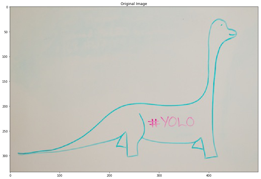
1 | # Load image |
2 | img_yolo = io.imread('imgs/yolo.jpg') |
3 | img_yolo = util.img_as_float(img_yolo) |
4 | |
5 | plt.title('Original Image') |
6 | plt.imshow(img_yolo) |
7 | plt.show() |
1 | from seam_carving import compute_forward_cost |
2 | |
3 | # Let's first test with a small example |
4 | img_test = np.array([[1.0, 1.0, 2.0], |
5 | [0.5, 0.0, 0.0], |
6 | [1.0, 0.5, 2.0]]) |
7 | img_test = np.stack([img_test]*3, axis=2) |
8 | assert img_test.shape == (3, 3, 3) |
9 | |
10 | energy = energy_function(img_test) |
11 | |
12 | solution_cost = np.array([[0.5, 2.5, 3.0], |
13 | [1.0, 2.0, 3.0], |
14 | [2.0, 4.0, 6.0]]) |
15 | |
16 | solution_paths = np.array([[ 0, 0, 0], |
17 | [ 0, -1, 0], |
18 | [ 0, -1, -1]]) |
19 | |
20 | # Vertical Cost Map |
21 | vcost, vpaths = compute_forward_cost(img_test, energy) # don't need the first argument for compute_cost |
22 | |
23 | print("Image:") |
24 | print(color.rgb2grey(img_test)) |
25 | |
26 | print("Energy:") |
27 | print(energy) |
28 | |
29 | print("Cost:") |
30 | print(vcost) |
31 | print("Solution cost:") |
32 | print(solution_cost) |
33 | |
34 | print("Paths:") |
35 | print(vpaths) |
36 | print("Solution paths:") |
37 | print(solution_paths) |
38 | |
39 | assert np.allclose(solution_cost, vcost) |
40 | assert np.allclose(solution_paths, vpaths) |
1 | from seam_carving import compute_forward_cost |
2 | |
3 | energy = energy_function(img_yolo) |
4 | |
5 | out, _ = compute_cost(img_yolo, energy) |
6 | plt.subplot(1, 2, 1) |
7 | plt.imshow(out, cmap='inferno') |
8 | plt.title("Normal cost function") |
9 | |
10 | out, _ = compute_forward_cost(img_yolo, energy) |
11 | plt.subplot(1, 2, 2) |
12 | plt.imshow(out, cmap='inferno') |
13 | plt.title("Forward cost function") |
14 | |
15 | plt.show() |
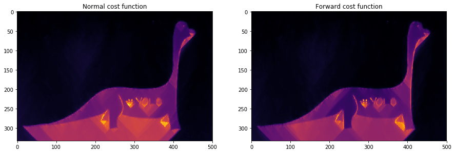
We observe that the forward energy insists more on the curved edges of the image.
可以看到,Forward Energy方法在保留边缘曲线的结构上比原方法好。
1 | from seam_carving import reduce |
2 | |
3 | start = time() |
4 | out = reduce(img_yolo, 200, axis=0) |
5 | end = time() |
6 | print("Old Solution: %f seconds." % (end - start)) |
7 | |
8 | plt.imshow(out) |
9 | plt.show() |
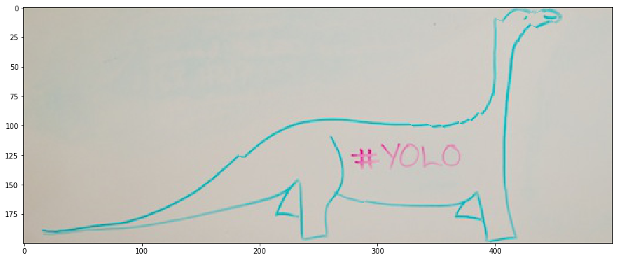
The issue with our standard reduce function is that it removes vertical seams without any concern for the energy introduced in the image.
In the case of the dinosaur above, the continuity of the shape is broken. The head is totally wrong for instance, and the back of the dinosaure lacks continuity.
Forward energy will solve this issue by explicitely putting high energy on a seam that breaks this continuity and introduces energy.
1 | # This step can take a very long time depending on your implementation. |
2 | start = time() |
3 | out = reduce(img_yolo, 200, axis=0, cfunc=compute_forward_cost) |
4 | end = time() |
5 | print("Forward Energy Solution: %f seconds." % (end - start)) |
6 | |
7 | plt.imshow(out) |
8 | plt.show() |

Object removal (extra credit 0.5%)
Object removal uses a binary mask of the object to be removed.
Using the reduce and enlarge functions you wrote before, complete the function remove_object to output an image of the same shape but without the object to remove.
移除目标和保留目标
移除目标的思路应该很清晰,就是将图像中目标处的像素视为能量最小或最大,即可将目标去除了。
两个问题:
- 如何进行标记,从而每次删除能量线的时候,都能删到并且尽可能多的删到带有标记的能量线?同时坐标下标不会混乱。
- 如何在删除目标之后保持和原图同样的尺寸
解决方式:
- 判断最小能量线的时候,将mask区域乘上负数,自然找到的接缝能量会最小,并且穿过mask区域的像素点会更多。
- 做裁剪的时候,将mask根据接缝和图像一起进行裁剪,自然不会引起下标混乱。
- 删除目标之后再调用之前的enlarge函数,进行图像的放大,放大到原图尺寸。
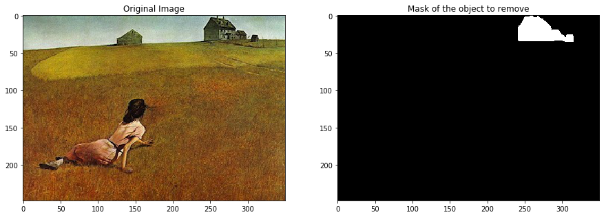
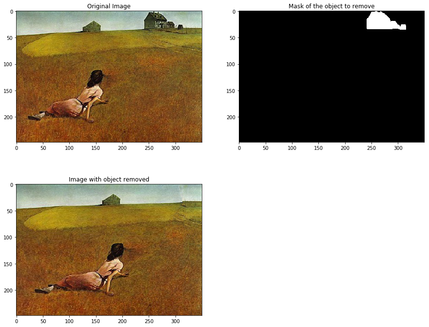
1 | # Load image |
2 | image = io.imread('imgs/wyeth.jpg') |
3 | image = util.img_as_float(image) |
4 | |
5 | mask = io.imread('imgs/wyeth_mask.jpg', as_grey=True) |
6 | mask = util.img_as_bool(mask) |
7 | |
8 | plt.subplot(1, 2, 1) |
9 | plt.title('Original Image') |
10 | plt.imshow(image) |
11 | |
12 | plt.subplot(1, 2, 2) |
13 | plt.title('Mask of the object to remove') |
14 | plt.imshow(mask) |
15 | |
16 | plt.show() |
1 | # Use your function to remove the object |
2 | from seam_carving import remove_object |
3 | out = remove_object(image, mask) |
4 | |
5 | plt.subplot(2, 2, 1) |
6 | plt.title('Original Image') |
7 | plt.imshow(image) |
8 | |
9 | plt.subplot(2, 2, 2) |
10 | plt.title('Mask of the object to remove') |
11 | plt.imshow(mask) |
12 | |
13 | plt.subplot(2, 2, 3) |
14 | plt.title('Image with object removed') |
15 | plt.imshow(out) |
16 | |
17 | plt.show() |
Segmentation-Clustering
实现聚类算法:K-Means和HAC(凝聚聚类算法);
构建图像的特征序列,进行聚类分割;
实现分割结果与GroundTruth的量化评估,根据指标评估聚类算法。
This notebook includes both coding and written questions. Please hand in this notebook file with all the outputs and your answers to the written questions.
This assignment covers K-Means and HAC methods for clustering.
这份作业包含的主题:用于聚类的K-means 和 HAC(层次凝聚聚类)方法,以及聚类算法的量化评估。
Introduction
In this assignment, you will use clustering algorithms to segment images. You will then use these segmentations to identify foreground and background objects.
Your assignment will involve the following subtasks:
- Clustering algorithms: Implement K-Means clustering and Hierarchical Agglomerative Clustering.
- Pixel-level features: Implement a feature vector that combines color and position information and implement feature normalization.
- Quantitative Evaluation: Evaluate segmentation algorithms with a variety of parameter settings by comparing your computed segmentations against a dataset of ground-truth segmentations.
Clustering Algorithms
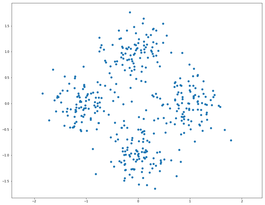
1 | # Generate random data points for clustering |
2 | |
3 | # Cluster 1 |
4 | mean1 = [-1, 0] |
5 | cov1 = [[0.1, 0], [0, 0.1]] |
6 | X1 = np.random.multivariate_normal(mean1, cov1, 100) |
7 | |
8 | # Cluster 2 |
9 | mean2 = [0, 1] |
10 | cov2 = [[0.1, 0], [0, 0.1]] |
11 | X2 = np.random.multivariate_normal(mean2, cov2, 100) |
12 | |
13 | # Cluster 3 |
14 | mean3 = [1, 0] |
15 | cov3 = [[0.1, 0], [0, 0.1]] |
16 | X3 = np.random.multivariate_normal(mean3, cov3, 100) |
17 | |
18 | # Cluster 4 |
19 | mean4 = [0, -1] |
20 | cov4 = [[0.1, 0], [0, 0.1]] |
21 | X4 = np.random.multivariate_normal(mean4, cov4, 100) |
22 | |
23 | # Merge two sets of data points |
24 | X = np.concatenate((X1, X2, X3, X4)) |
25 | |
26 | # Plot data points |
27 | plt.scatter(X[:, 0], X[:, 1]) |
28 | plt.axis('equal') |
29 | plt.show() |
K-Means Clustering
As discussed in class, K-Means is one of the most popular clustering algorithms. We have provided skeleton code for K-Means clustering in the file segmentation.py. Your first task is to finish implementing kmeans in segmentation.py. This version uses nested for loops to assign points to the closest centroid and compute new mean of each cluster.
目前题图允许使用循环实现点到最近中心的分配即可。
K-means的步骤:
- 随机初始化聚类中心
- 将点分配给最近的中心
- 计算每个聚类的新的中心
- 如果聚类的分配不再变动则停止
- 从第二步继续循环
1 | from segmentation import kmeans |
2 | |
3 | np.random.seed(0) |
4 | start = time() |
5 | assignments = kmeans(X, 4) |
6 | end = time() |
7 | |
8 | kmeans_runtime = end - start |
9 | |
10 | print("kmeans running time: %f seconds." % kmeans_runtime) |
11 | |
12 | for i in range(4): |
13 | cluster_i = X[assignments==i] |
14 | plt.scatter(cluster_i[:, 0], cluster_i[:, 1]) |
15 | |
16 | plt.axis('equal') |
17 | plt.show() |
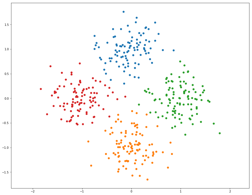
简单的实现了K-Means算法,第三步判断终止条件很重要,添加终止条件后只迭代了几次就结束了,大大降低了运行时间。
We can use numpy functions and broadcasting to make kmeans faster. Implement kmeans_fast in segmentation.py. This should run at least 10 times faster than the previous implementation.
思路:
题目的提示是使用numpy函数和broadcasting机制
np.repeat and np.argmin 有帮助
还有一种思路就是向量化了,不做迭代而是放在矩阵里去计算。
1 | from segmentation import kmeans_fast |
2 | |
3 | np.random.seed(0) |
4 | start = time() |
5 | assignments = kmeans_fast(X, 4) |
6 | end = time() |
7 | |
8 | kmeans_fast_runtime = end - start |
9 | print("kmeans running time: %f seconds." % kmeans_fast_runtime) |
10 | print("%f times faster!" % (kmeans_runtime / kmeans_fast_runtime)) |
11 | |
12 | for i in range(4): |
13 | cluster_i = X[assignments==i] |
14 | plt.scatter(cluster_i[:, 0], cluster_i[:, 1]) |
15 | |
16 | plt.axis('equal') |
17 | plt.show() |

快了十六倍 ,666,向量化是个好东西!!!
Hierarchical Agglomerative Clustering
Another simple clustering algorithm is Hieararchical Agglomerative Clustering, which is somtimes abbreviated as HAC. In this algorithm, each point is initially assigned to its own cluster. Then cluster pairs are merged until we are left with the desired number of predetermined clusters (see Algorithm 1).
Implement hiererachical_clustering in segmentation.py.
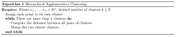
按照上图的算法定义是:
- 初始化每个点为一个簇
- 迭代直到只剩下K个簇:
- 计算所有簇与簇之间(簇对)的距离
- 合并最近的两个簇
这个算法的关键,主要是如何定义簇与簇之间的距离。定义有下面三种:
- 单链(Single-link):不同两个聚类中离得最近的两个点之间的距离,即MIN;
- 全链(Complete-link):不同两个聚类中离得最远的两个点之间的距离,即MAX;
- 平均链(Average-link):不同两个聚类中所有点对距离的平均值,即AVERAGE;
题目代码中提示的做法是,利用簇中心的欧几里得距离来定义簇与簇之间的距离。
hierarchical_clustering函数将按照这个思路实现。
Numpy中的距离度量函数: 距离度量以及python实现(一)
1 | from segmentation import hierarchical_clustering |
2 | |
3 | start = time() |
4 | assignments = hierarchical_clustering(X, 4) |
5 | end = time() |
6 | |
7 | print("hierarchical_clustering running time: %f seconds." % (end - start)) |
8 | |
9 | for i in range(4): |
10 | cluster_i = X[assignments==i] |
11 | plt.scatter(cluster_i[:, 0], cluster_i[:, 1]) |
12 | |
13 | plt.axis('equal') |
14 | plt.show() |
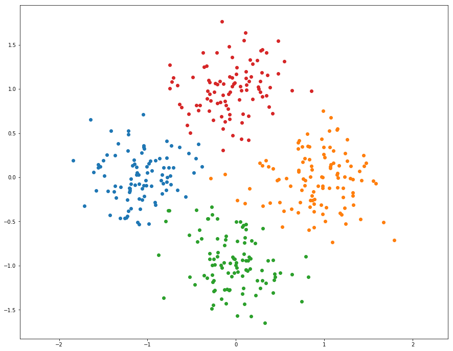
运行时间比预期的块,总结一下就是这类算法的提速方式:
- 第一个是善用向量化,用矩阵来计算问题
- 第二个就是善用numpy提供的函数,解决一些需要搜索遍历的问题
Pixel-Level Features
Before we can use a clustering algorithm to segment an image, we must compute some feature vectore for each pixel. The feature vector for each pixel should encode the qualities that we care about in a good segmentation. More concretely, for a pair of pixels and with corresponding feature vectors and , the distance between and should be small if we believe that and should be placed in the same segment and large otherwise.
上一步的聚类算法实现其实是流程的第二步,第一步其实是特征的提取,有了特征才能进行像素(或者说样本)的聚类。只不过第一步中,拿了点的位置作为特征来进行聚类了。
1 | # Load and display image |
2 | img = io.imread('train.jpg') |
3 | H, W, C = img.shape |
4 | |
5 | plt.imshow(img) |
6 | plt.axis('off') |
7 | plt.show() |
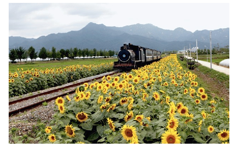
Color Features
One of the simplest possible feature vectors for a pixel is simply the vector of colors for that pixel. Implement color_features in segmentation.py. Output should look like the following:
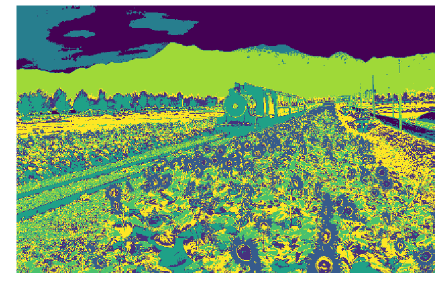
在color_features实现简单的颜色特征的聚类。
1 | from segmentation import color_features |
2 | np.random.seed(0) |
3 | |
4 | features = color_features(img) |
5 | |
6 | # Sanity checks |
7 | assert features.shape == (H * W, C),\ |
8 | "Incorrect shape! Check your implementation." |
9 | |
10 | assert features.dtype == np.float,\ |
11 | "dtype of color_features should be float." |
12 | |
13 | assignments = kmeans_fast(features, 8) |
14 | segments = assignments.reshape((H, W)) |
15 | |
16 | # Display segmentation |
17 | plt.imshow(segments, cmap='viridis') |
18 | plt.axis('off') |
19 | plt.show() |
In the cell below, we visualize each segment as the mean color of pixels in the segment.
将聚类结果用颜色进行显示(颜色是指源图各个分割区域内的颜色均值)
1 | from utils import visualize_mean_color_image |
2 | visualize_mean_color_image(img, segments) |
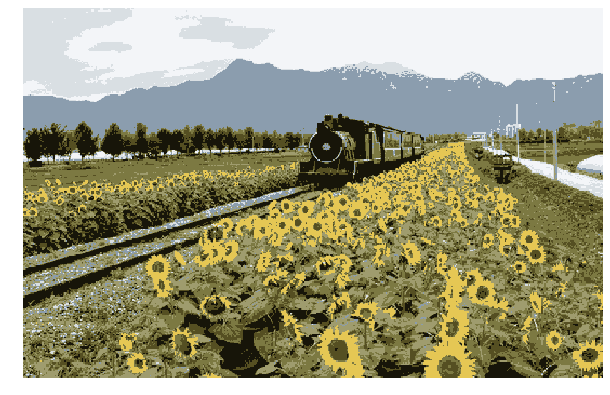
Color and Position Features
Another simple feature vector for a pixel is to concatenate its color and position within the image. In other words, for a pixel of color located at position in the image, its feature vector would be . However, the color and position features may have drastically different ranges; for example each color channel of an image may be in the range , while the position of each pixel may have a much wider range. Uneven scaling between different features in the feature vector may cause clustering algorithms to behave poorly.
One way to correct for uneven scaling between different features is to apply some sort of normalization to the feature vector. One of the simplest types of normalization is to force each feature to have zero mean and unit variance.
Implement color_position_features in segmentation.py.
Output segmentation should look like the following:

结合颜色特征和位置特征的聚类
其实就是生成特征为 的序列,但需要考虑的问题是尺度的不同,解决的方案也很简单,就是进行归一化,对每一个维度进行归一化。公式如下:
1 | from segmentation import color_position_features |
2 | np.random.seed(0) |
3 | |
4 | features = color_position_features(img) |
5 | |
6 | # Sanity checks |
7 | assert features.shape == (H * W, C + 2),\ |
8 | "Incorrect shape! Check your implementation." |
9 | |
10 | assert features.dtype == np.float,\ |
11 | "dtype of color_features should be float." |
12 | |
13 | assignments = kmeans_fast(features, 8) |
14 | segments = assignments.reshape((H, W)) |
15 | |
16 | # Display segmentation |
17 | plt.imshow(segments, cmap='viridis') |
18 | plt.axis('off') |
19 | plt.show() |
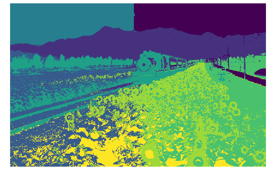
1 | visualize_mean_color_image(img, segments) |
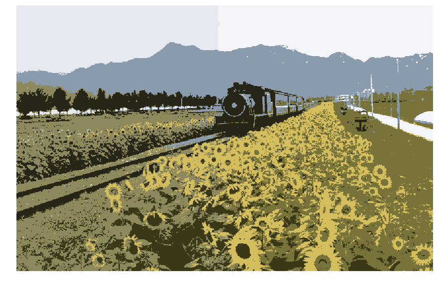
Extra Credit: Implement Your Own Feature
For this programming assignment we have asked you to implement a very simple feature transform for each pixel. While it is not required, you should feel free to experiment with other feature transforms. Could your final segmentations be improved by adding gradients, edges, SIFT descriptors, or other information to your feature vectors? Could a different type of normalization give better results?
Implement your feature extractor my_features in segmentation.py
Depending on the creativity of your approach and the quality of your writeup, implementing extra feature vectors can be worth extra credit (up to 5% of total points).
Describe your approach: (YOUR APPROACH)
实现自己定义的特征
可以实现一些简单的特征,比如添加梯度、边缘、SIFT描述子或者其他信息。
我添加了一个梯度强度信息,结合颜色特征,位置特征。
1 | from segmentation import my_features |
2 | |
3 | # Feel free to experiment with different images |
4 | # and varying number of segments |
5 | img = io.imread('train.jpg') |
6 | num_segments = 8 |
7 | |
8 | H, W, C = img.shape |
9 | |
10 | # Extract pixel-level features |
11 | features = my_features(img) |
12 | |
13 | # Run clustering algorithm |
14 | assignments = kmeans_fast(features, num_segments) |
15 | |
16 | segments = assignments.reshape((H, W)) |
17 | |
18 | # Display segmentation |
19 | plt.imshow(segments, cmap='viridis') |
20 | plt.axis('off') |
21 | plt.show() |

Quantitative Evaluation
Looking at images is a good way to get an idea for how well an algorithm is working, but the best way to evaluate an algorithm is to have some quantitative measure of its performance.
For this project we have supplied a small dataset of cat images and ground truth segmentations of these images into foreground (cats) and background (everything else). We will quantitatively evaluate different segmentation methods (features and clustering methods) on this dataset.
We can cast the segmentation task into a binary classification problem, where we need to classify each pixel in an image into either foreground (positive) or background (negative). Given the ground-truth labels, the accuracy of a segmentation is (TP+TN)/(P+N).
Implement compute_accuracy in segmentation.py.
实现准确率计算就是正确个数与总个数之比。
1 | from segmentation import compute_accuracy |
2 | |
3 | mask_gt = np.zeros((100, 100)) |
4 | mask = np.zeros((100, 100)) |
5 | |
6 | # Test compute_accracy function |
7 | mask_gt[20:50, 30:60] = 1 |
8 | mask[30:50, 30:60] = 1 |
9 | |
10 | accuracy = compute_accuracy(mask_gt, mask) |
11 | |
12 | print('Accuracy: %0.2f' % (accuracy)) |
13 | if accuracy != 0.97: |
14 | print('Check your implementation!') |
15 | |
16 | plt.subplot(121) |
17 | plt.imshow(mask_gt) |
18 | plt.title('Ground Truth') |
19 | plt.axis('off') |
20 | |
21 | plt.subplot(122) |
22 | plt.imshow(mask) |
23 | plt.title('Estimate') |
24 | plt.axis('off') |
25 | |
26 | plt.show() |
You can use the script below to evaluate a segmentation method’s ability to separate foreground from background on the entire provided dataset. Use this script as a starting point to evaluate a variety of segmentation parameters.
下面这段程序是已经完成的,主要逻辑就是
- 加载数据集,包括原图和分割结果真值
- 调用之前实现的聚类分割算法进行分割
- 将真值和分割结果进行比对,计算准确率
可以在下面进行调参,更改参数,查看效果。
1 | from utils import load_dataset, compute_segmentation |
2 | from segmentation import evaluate_segmentation,my_features |
3 | |
4 | # Load a small segmentation dataset |
5 | imgs, gt_masks = load_dataset('./data') |
6 | |
7 | # Set the parameters for segmentation. |
8 | num_segments = 3 |
9 | clustering_fn = kmeans_fast #hierarchical_clustering |
10 | feature_fn = color_position_features # color_features #color_position_features # my_features |
11 | scale =0.5 |
12 | |
13 | mean_accuracy = 0.0 |
14 | |
15 | segmentations = [] |
16 | |
17 | for i, (img, gt_mask) in enumerate(zip(imgs, gt_masks)): |
18 | # Compute a segmentation for this image |
19 | segments = compute_segmentation(img, num_segments, |
20 | clustering_fn=clustering_fn, |
21 | feature_fn=feature_fn, |
22 | scale=scale) |
23 | |
24 | segmentations.append(segments) |
25 | |
26 | # Evaluate segmentation |
27 | accuracy = evaluate_segmentation(gt_mask, segments) |
28 | |
29 | print('Accuracy for image %d: %0.4f' %(i, accuracy)) |
30 | mean_accuracy += accuracy |
31 | |
32 | mean_accuracy = mean_accuracy / len(imgs) |
33 | print('Mean accuracy: %0.4f' % mean_accuracy) |
1 | # Visualize segmentation results |
2 | |
3 | N = len(imgs) |
4 | plt.figure(figsize=(15,60)) |
5 | for i in range(N): |
6 | |
7 | plt.subplot(N, 3, (i * 3) + 1) |
8 | plt.imshow(imgs[i]) |
9 | plt.axis('off') |
10 | |
11 | plt.subplot(N, 3, (i * 3) + 2) |
12 | plt.imshow(gt_masks[i]) |
13 | plt.axis('off') |
14 | |
15 | plt.subplot(N, 3, (i * 3) + 3) |
16 | plt.imshow(segmentations[i], cmap='viridis') |
17 | plt.axis('off') |
18 | |
19 | plt.show() |
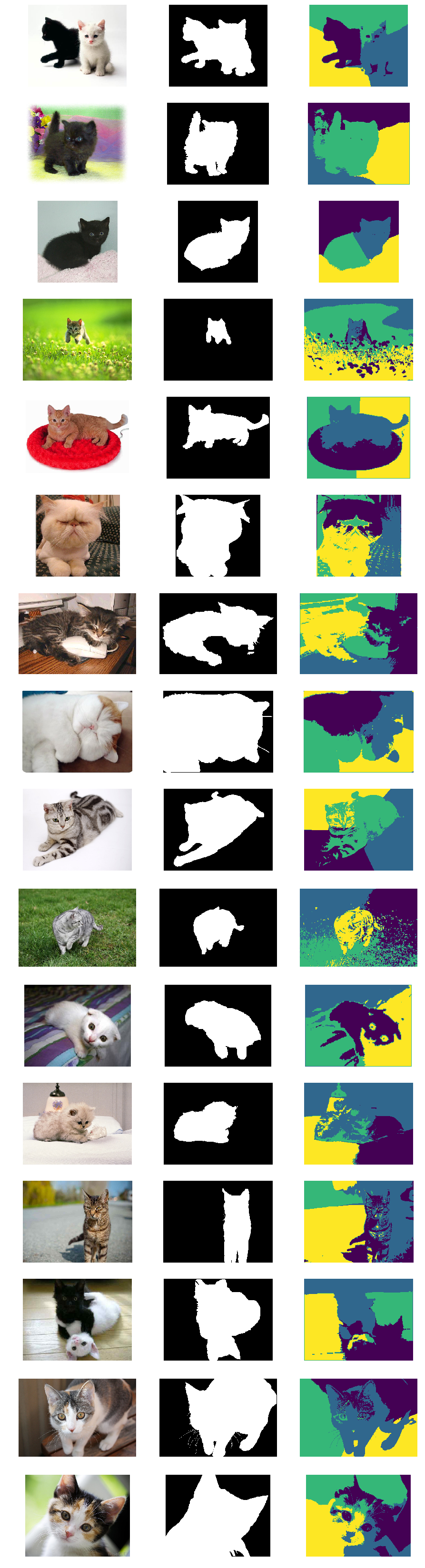
Include a detailed evaluation of the effect of varying segmentation parameters (feature transform, clustering method, number of clusters, resize) on the mean accuracy of foreground-background segmentations on the provided dataset. You should test a minimum of 10 combinations of parameters. To present your results, add rows to the table below (you may delete the first row).
Observe your results carefully and try to answer the following question:
- Based on your quantitative experiments, how do each of the segmentation parameters affect the quality of the final foreground-background segmentation?
- Are some images simply more difficult to segment correctly than others? If so, what are the qualities of these images that cause the segmentation algorithms to perform poorly?
- Also feel free to point out or discuss any other interesting observations that you made.
基于对结果的观察:
- 基于颜色-位置特征的聚类效果比基于颜色特征的聚类效果差
- 聚类数目3个就是最好的了,增大减小都影响效果
- 尺度是越接近原图,也就是越接近1,准确度越高
的确存在一些图更难识别。这些图的一些特性包括
- 背景较为复杂
- 前景颜色、亮度都与背景较为接近
同时基于颜色-位置特征的聚类中,尺度并不是越大越好,可能是我做的实验次数不够多。
Recognition-Classification
实现分类算法。
使用SVD进行图像压缩。
使用KNN进行图像识别(分类)。
使用PCA(主成分分析)和LDA(线性判别分析)对数据进行降维。
This notebook includes both coding and written questions. Please hand in this notebook file with all the outputs as a pdf on gradescope for “HW6 pdf”. Upload the three files of code (compression.py, k_nearest_neighbor.py and features.py) on gradescope for “HW6 code”.
This assignment covers:
- image compression using SVD
- kNN methods for image recognition.
- PCA and LDA to improve kNN
Image Compression
Image compression is used to reduce the cost of storage and transmission of images (or videos).
One lossy compression method is to apply Singular Value Decomposition (SVD) to an image, and only keep the top n singular values.
1 | image = io.imread('pitbull.jpg', as_grey=True) |
2 | plt.imshow(image) |
3 | plt.axis('off') |
4 | plt.show() |
Let’s implement image compression using SVD.
We first compute the SVD of the image, and as seen in class we keep the largest singular values and singular vectors to reconstruct the image.
Implement function compress_image in compression.py.
在compress_image函数中实现奇异值分解,并保留前N个较大的奇异值和对应的特征向量。
题目中的压缩率在我理解就是压缩后有效数据与压缩之前图像数据的比值。
1 | from compression import compress_image |
2 | |
3 | compressed_image, compressed_size = compress_image(image, 100) |
4 | compression_ratio = compressed_size / image.size |
5 | print('Original image shape:', image.shape) |
6 | print('Compressed size: %d' % compressed_size) |
7 | print('Compression ratio: %.3f' % compression_ratio) |
8 | |
9 | assert compressed_size == 298500 |
1 | Original image shape: (1704, 1280) |
2 | Compressed size: 298500 |
3 | Compression ratio: 0.137 |
1 | # Number of singular values to keep |
2 | n_values = [10, 50, 100] |
3 | |
4 | for n in n_values: |
5 | # Compress the image using `n` singular values |
6 | compressed_image, compressed_size = compress_image(image, n) |
7 | |
8 | compression_ratio = compressed_size / image.size |
9 | |
10 | print("Data size (original): %d" % (image.size)) |
11 | print("Data size (compressed): %d" % compressed_size) |
12 | print("Compression ratio: %f" % (compression_ratio)) |
13 | |
14 | |
15 | |
16 | plt.imshow(compressed_image, cmap='gray') |
17 | title = "n = %s" % n |
18 | plt.title(title) |
19 | plt.axis('off') |
20 | plt.show() |
1 | Data size (original): 2181120 |
2 | Data size (compressed): 29850 |
3 | Compression ratio: 0.013686 |
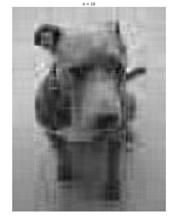
1 | Data size (original): 2181120 |
2 | Data size (compressed): 149250 |
3 | Compression ratio: 0.068428 |
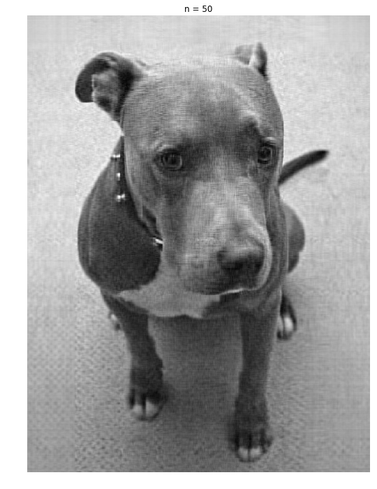
1 | Data size (original): 2181120 |
2 | Data size (compressed): 298500 |
3 | Compression ratio: 0.136856 |

实现了用SVD实现了图像的压缩,同时可以发现:n=100时,压缩率0.13时,图像质量就已经很接近原图了。
这样看来,SVD的确用来做降维是很合适的。毕竟能够大大提高运行速度。
Face Dataset
We will use a dataset of faces of celebrities. Download the dataset using the following command:
1 | sh get_dataset.sh |
The face dataset for CS131 assignment.
The directory containing the dataset has the following structure:
1 | faces/ |
2 | train/ |
3 | angelina jolie/ |
4 | anne hathaway/ |
5 | ... |
6 | test/ |
7 | angelina jolie/ |
8 | anne hathaway/ |
9 | ... |
Each class has 50 training images and 10 testing images.
命令行执行sh get_dataset.sh就可以下载了。
1 | # 加载数据集 |
2 | from utils import load_dataset |
3 | |
4 | X_train, y_train, classes_train = load_dataset('faces', train=True, as_grey=True) |
5 | X_test, y_test, classes_test = load_dataset('faces', train=False, as_grey=True) |
6 | |
7 | assert classes_train == classes_test |
8 | classes = classes_train |
9 | |
10 | print('Class names:', classes) |
11 | print('Training data shape:', X_train.shape) |
12 | print('Training labels shape: ', y_train.shape) |
13 | print('Test data shape:', X_test.shape) |
14 | print('Test labels shape: ', y_test.shape) |
1 | Class names: ['angelina jolie', 'anne hathaway', 'barack obama', 'brad pitt', 'cristiano ronaldo', 'emma watson', 'george clooney', 'hillary clinton', 'jennifer aniston', 'johnny depp', 'justin timberlake', 'leonardo dicaprio', 'natalie portman', 'nicole kidman', 'scarlett johansson', 'tom cruise'] |
2 | Training data shape: (800, 64, 64) |
3 | Training labels shape: (800,) |
4 | Test data shape: (160, 64, 64) |
5 | Test labels shape: (160,) |
1 | # 可视化数据集中的一些样本 |
2 | # 从每一类中显示一些样本 |
3 | num_classes = len(classes) |
4 | samples_per_class = 10 |
5 | for y, cls in enumerate(classes): |
6 | idxs = np.flatnonzero(y_train == y) |
7 | idxs = np.random.choice(idxs, samples_per_class, replace=False) |
8 | for i, idx in enumerate(idxs): |
9 | plt_idx = i * num_classes + y + 1 |
10 | plt.subplot(samples_per_class, num_classes, plt_idx) |
11 | plt.imshow(X_train[idx]) |
12 | plt.axis('off') |
13 | if i == 0: |
14 | plt.title(y) |
15 | plt.show() |
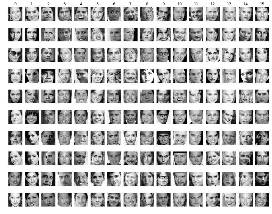
1 | # 将图像数据展开为行,即每个样本为一行 |
2 | # 这样每个样本我们就有了4096个维度的特征 |
3 | X_train = np.reshape(X_train, (X_train.shape[0], -1)) |
4 | X_test = np.reshape(X_test, (X_test.shape[0], -1)) |
5 | print("Training data shape:", X_train.shape) |
6 | print("Test data shape:", X_test.shape) |
1 | Training data shape: (800, 4096) |
2 | Test data shape: (160, 4096) |
k-Nearest Neighbor
We’re now going to try to classify the test images using the k-nearest neighbors algorithm on the raw features of the images (i.e. the pixel values themselves). We will see later how we can use kNN on better features.
Here are the steps that we will follow:
- We compute the L2 distances between every element of X_test and every element of X_train in
compute_distances - We split the dataset into 5 folds for cross-validation in
split_folds. - For each fold, and for different values of
k, we predict the labels and measure accuracy. - Using the best
kfound through cross-validation, we measure accuracy on the test set.
kNN(k最近邻算法)的步骤如下:
- 计算测试数据X_test中每个样本与训练数据X_train中每个样本之间的距离,距离计算方式为L2距离。
- 将数据集分割为5Folder(5折)
- 对每个子集和每个不同的参数k,预测结果并计算准确率
- 通过交叉验证找到最佳的参数k,并在测试集上评估准确率
1 | from k_nearest_neighbor import compute_distances |
2 | |
3 | # Step 1: compute the distances between all features from X_train and from X_test |
4 | # 第一步:计算训练集和测试集上所有特征的距离(L2),调用cdist函数即可 |
5 | dists = compute_distances(X_test, X_train) |
6 | assert dists.shape == (160, 800) |
7 | print("dists shape:", dists.shape) |
1 | dists shape: (160, 800) |
预测结果分两步:
- 找到预测点的最近的k个点
- 判断k个点中频率最高的train_label
1 | from k_nearest_neighbor import predict_labels |
2 | |
3 | # We use k = 1 (which corresponds to only taking the nearest neighbor to decide) |
4 | y_test_pred = predict_labels(dists, y_train, k=1) |
5 | |
6 | # Compute and print the fraction of correctly predicted examples |
7 | num_test = y_test.shape[0] |
8 | num_correct = np.sum(y_test_pred == y_test) |
9 | accuracy = float(num_correct) / num_test |
10 | print('Got %d / %d correct => accuracy: %f' % (num_correct, num_test, accuracy)) |
1 | Got 38 / 160 correct => accuracy: 0.237500 |
Cross-Validation
We don’t know the best value for our parameter k.
There is no theory on how to choose an optimal k, and the way to choose it is through cross-validation.
We cannot compute any metric on the test set to choose the best k, because we want our final test accuracy to reflect a real use case. This real use case would be a setting where we have new examples come and we classify them on the go. There is no way to check the accuracy beforehand on that set of test examples to determine k.
Cross-validation will make use split the data into different fold (5 here).
For each fold, if we have a total of 5 folds we will have:
- 80% of the data as training data
- 20% of the data as validation data
We will compute the accuracy on the validation accuracy for each fold, and use the mean of these 5 accuracies to determine the best parameter k.
1 | from k_nearest_neighbor import split_folds |
2 | |
3 | # Step 2: split the data into 5 folds to perform cross-validation. |
4 | # 步骤二:分割数据为5折,执行交叉验证 |
5 | num_folds = 5 |
6 | |
7 | X_trains, y_trains, X_vals, y_vals = split_folds(X_train, y_train, num_folds) |
8 | |
9 | assert X_trains.shape == (5, 640, 4096) |
10 | assert y_trains.shape == (5, 640) |
11 | assert X_vals.shape == (5, 160, 4096) |
12 | assert y_vals.shape == (5, 160) |
1 | # Step 3: Measure the mean accuracy for each value of `k` |
2 | # 步骤三:计算每个参数k对应的平均准确率 |
3 | |
4 | # List of k to choose from |
5 | k_choices = list(range(5, 101, 5)) |
6 | |
7 | # Dictionnary mapping k values to accuracies |
8 | # For each k value, we will have `num_folds` accuracies to compute |
9 | # k_to_accuracies[1] will be for instance [0.22, 0.23, 0.19, 0.25, 0.20] for 5 folds |
10 | k_to_accuracies = {} |
11 | |
12 | for k in k_choices: |
13 | print("Running for k=%d" % k) |
14 | accuracies = [] |
15 | for i in range(num_folds): |
16 | # Make predictions |
17 | fold_dists = compute_distances(X_vals[i], X_trains[i]) |
18 | y_pred = predict_labels(fold_dists, y_trains[i], k) |
19 | |
20 | # Compute and print the fraction of correctly predicted examples |
21 | num_correct = np.sum(y_pred == y_vals[i]) |
22 | accuracy = float(num_correct) / len(y_vals[i]) |
23 | accuracies.append(accuracy) |
24 | |
25 | k_to_accuracies[k] = accuracies |
1 | # plot the raw observations |
2 | # 绘图进行观察 |
3 | for k in k_choices: |
4 | accuracies = k_to_accuracies[k] |
5 | plt.scatter([k] * len(accuracies), accuracies) |
6 | |
7 | # plot the trend line with error bars that correspond to standard deviation |
8 | # |
9 | accuracies_mean = np.array([np.mean(v) for k,v in sorted(k_to_accuracies.items())]) |
10 | accuracies_std = np.array([np.std(v) for k,v in sorted(k_to_accuracies.items())]) |
11 | plt.errorbar(k_choices, accuracies_mean, yerr=accuracies_std) |
12 | plt.title('Cross-validation on k') |
13 | plt.xlabel('k') |
14 | plt.ylabel('Cross-validation accuracy') |
15 | plt.show() |
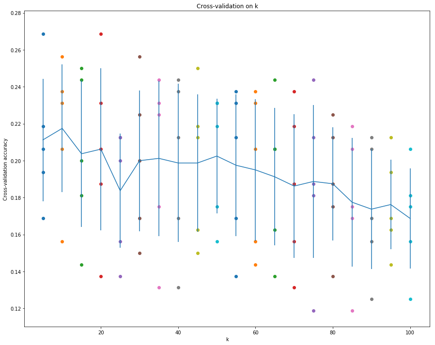
从这幅图看,前30之内有两个峰值就达到了最高的准确率和较好的标准差。
可以进一步细化step进行测试。
1 | # Step 3: Measure the mean accuracy for each value of `k` |
2 | # 步骤三:计算每个参数k对应的平均准确率 |
3 | |
4 | # List of k to choose from |
5 | k_choices = list(range(1, 31, 1)) |
6 | |
7 | # Dictionnary mapping k values to accuracies |
8 | # For each k value, we will have `num_folds` accuracies to compute |
9 | # k_to_accuracies[1] will be for instance [0.22, 0.23, 0.19, 0.25, 0.20] for 5 folds |
10 | k_to_accuracies = {} |
11 | |
12 | for k in k_choices: |
13 | print("Running for k=%d" % k) |
14 | accuracies = [] |
15 | for i in range(num_folds): |
16 | # Make predictions |
17 | fold_dists = compute_distances(X_vals[i], X_trains[i]) |
18 | y_pred = predict_labels(fold_dists, y_trains[i], k) |
19 | |
20 | # Compute and print the fraction of correctly predicted examples |
21 | num_correct = np.sum(y_pred == y_vals[i]) |
22 | accuracy = float(num_correct) / len(y_vals[i]) |
23 | accuracies.append(accuracy) |
24 | |
25 | k_to_accuracies[k] = accuracies |
1 | # plot the raw observations |
2 | # 绘图进行观察 |
3 | for k in k_choices: |
4 | accuracies = k_to_accuracies[k] |
5 | plt.scatter([k] * len(accuracies), accuracies) |
6 | |
7 | # plot the trend line with error bars that correspond to standard deviation |
8 | # |
9 | accuracies_mean = np.array([np.mean(v) for k,v in sorted(k_to_accuracies.items())]) |
10 | accuracies_std = np.array([np.std(v) for k,v in sorted(k_to_accuracies.items())]) |
11 | plt.errorbar(k_choices, accuracies_mean, yerr=accuracies_std) |
12 | plt.title('Cross-validation on k') |
13 | plt.xlabel('k') |
14 | plt.ylabel('Cross-validation accuracy') |
15 | plt.show() |
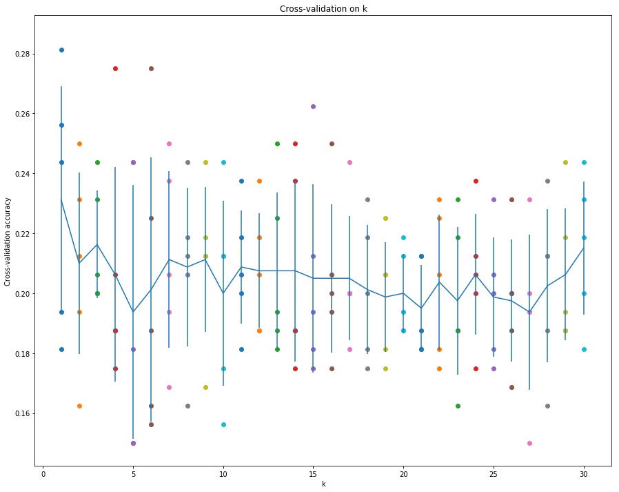
1 | # Based on the cross-validation results above, choose the best value for k, |
2 | # retrain the classifier using all the training data, and test it on the test |
3 | # data. You should be able to get above 26% accuracy on the test data. |
4 | |
5 | best_k = None |
6 | # YOUR CODE HERE |
7 | # Choose the best k based on the cross validation above |
8 | best_k =2 |
9 | # END YOUR CODE |
10 | |
11 | y_test_pred = predict_labels(dists, y_train, k=best_k) |
12 | |
13 | # Compute and display the accuracy |
14 | num_correct = np.sum(y_test_pred == y_test) |
15 | accuracy = float(num_correct) / num_test |
16 | print('For k = %d, got %d / %d correct => accuracy: %f' % (best_k, num_correct, num_test, accuracy)) |
1 | For k = 2, got 42 / 160 correct => accuracy: 0.262500 |
既然k=2和k=17准确率相同,应该是选择k较小的,这样可以提高运行速率吧。
PCA
Principal Component Analysis (PCA) is a simple yet popular and useful linear transformation technique that is used in numerous applications, such as stock market predictions, the analysis of gene expression data, and many more. In this tutorial, we will see that PCA is not just a “black box”, and we are going to unravel its internals in 3 basic steps.
Introduction
The sheer size of data in the modern age is not only a challenge for computer hardware but also a main bottleneck for the performance of many machine learning algorithms. The main goal of a PCA analysis is to identify patterns in data; PCA aims to detect the correlation between variables. If a strong correlation between variables exists, the attempt to reduce the dimensionality only makes sense. In a nutshell, this is what PCA is all about: Finding the directions of maximum variance in high-dimensional data and project it onto a smaller dimensional subspace while retaining most of the information.
A Summary of the PCA Approach
- Standardize the data.
- Obtain the Eigenvectors and Eigenvalues from the covariance matrix or correlation matrix, or perform Singular Vector Decomposition.
- Sort eigenvalues in descending order and choose the k eigenvectors that correspond to the k largest eigenvalues where k is the number of dimensions of the new feature subspace (k≤d).
- Construct the projection matrix from the selected k eigenvectors.
- Transform the original dataset via to obtain a -dimensional feature subspace Y.
PCA的主旨就是:在高维数据中找到最大方差的方向,并将高维数据投射到低维的子空间,这样能够保留尽可能多的信息。
- 标准化数据
- 从协方差矩阵或互相关矩阵或者用SVD奇异值分解,来获得特征向量和特征值
- 将特征值降序排序,根据新特征空间的维度k,选择前k个最大的特征值和对应的特征向量(k <= d)
- 根据k个特征向量构建投影矩阵W
- 将数据集X通过W转换到k维的特征子空间
1 | from features import PCA |
2 | pca = PCA() |
Eigendecomposition
The eigenvectors and eigenvalues of a covariance (or correlation) matrix represent the “core” of a PCA: The eigenvectors (principal components) determine the directions of the new feature space, and the eigenvalues determine their magnitude. In other words, the eigenvalues explain the variance of the data along the new feature axes.
Implement _eigen_decomp in pca.py.
特征向量和特征值代表了PCA的核心:
- 特征向量(主成分)决定了新的特征空间的方向
- 特征值决定了特征向量的幅度,换言之,特征值表示了数据在新特征方向的方差。方差越大,信息量越大。
1 | # Perform eigenvalue decomposition on the covariance matrix of training data. |
2 | # 在训练数据的协方差矩阵上执行特征分解 |
3 | t1 = time() |
4 | e_vecs, e_vals = pca._eigen_decomp(X_train - X_train.mean(axis=0)) |
5 | t2 = time() |
6 | |
7 | print(e_vals.shape) |
8 | print(e_vecs.shape) |
9 | print("耗时:", t2-t1) |
1 | (4096,) |
2 | (4096, 4096) |
3 | 耗时: 32.20034837722778 |
直接解特征向量太慢了。
Singular Value Decomposition
Doing an eigendecomposition of the covariance matrix is very expensive, especially when the number of features (D = 4096 here) gets very high.
To obtain the same eigenvalues and eigenvectors in a more efficient way, we can use Singular Value Decomposition (SVD). If we perform SVD on matrix , we obtain , and such that:
- the columns of U are the eigenvectors of
- the columns of VT are the eigenvectors of
- the values of S are the square roots of the eigenvalues of
Therefore, we can find out the top k eigenvectors of the covariance matrix using SVD.
Implement _svd in pca.py.
这里讲到了直接利用协方差矩阵计算特征分解是非常耗时的事情,特别是维度很高的情况下。
其实更高效的方式是使用SVD(奇异值分解)。
具体的左奇异向量和右奇异向量与特征向量的对应关系在上面描述了,所以利用SVD就能得到特征向量和特征值
1 | # Perform SVD on directly on the training data. |
2 | t1 = time() |
3 | u, s = pca._svd(X_train - X_train.mean(axis=0)) |
4 | t2 = time() |
5 | |
6 | print(s.shape) |
7 | print(u.shape) |
8 | print("耗时:", t2-t1) |
1 | (800,) |
2 | (4096, 4096) |
3 | 耗时: 1.3446221351623535 |
1 | # Test whether the square of singular values and eigenvalues are the same. |
2 | # We also observe that `e_vecs` and `u` are the same (only the sign of each column can differ). |
3 | # 这里测试直接分解协方差矩阵和使用SVD方法得到的是否相同 |
4 | N = X_train.shape[0] |
5 | assert np.allclose((s ** 2) / (N - 1), e_vals[:len(s)]) |
6 | |
7 | for i in range(len(s) - 1): |
8 | assert np.allclose(e_vecs[:, i], u[:, i]) or np.allclose(e_vecs[:, i], -u[:, i]) |
9 | # (the last eigenvector for i = len(s) - 1 is very noisy because the eigenvalue is almost 0, |
10 | # so imprecisions in the computation build up) |
Dimensionality Reduction
The top k principal components explain most of the variance of the underlying data.
By projecting our initial data (the images) onto the subspace spanned by the top k principal components,
we can reduce the dimension of our inputs while keeping most of the information.
In the example below, we can see that using the first two components in PCA is not enough to allow us to see pattern in the data. All the classes seem placed at random in the 2D plane.
维度缩减
通过将前k个主成分投影在子空间,就可以达到缩减维度的目的,同时能够保留最大的信息。
需要在feature.py中实现 transform 函数,同时在fit函数中实现X的均值计算
1 | # Dimensionality reduction by projecting the data onto |
2 | # lower dimensional subspace spanned by k principal components |
3 | |
4 | # To visualize, we will project in 2 dimensions |
5 | n_components = 2 |
6 | pca.fit(X_train) |
7 | X_proj = pca.transform(X_train, n_components) |
8 | |
9 | # Plot the top two principal components |
10 | for y in np.unique(y_train): |
11 | plt.scatter(X_proj[y_train==y,0], X_proj[y_train==y,1], label=classes[y]) |
12 | |
13 | plt.xlabel('1st component') |
14 | plt.ylabel('2nd component') |
15 | plt.legend() |
16 | plt.show() |
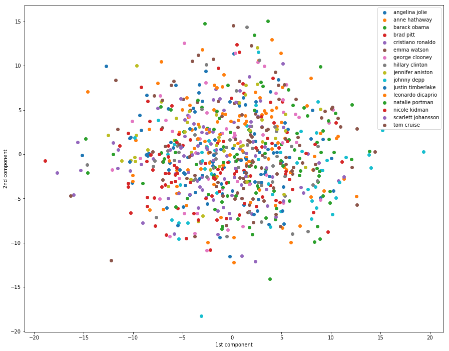
一脸懵逼,这里我们可以看到,仅仅用两个最大的主成分是无法看出数据的特征来的。
Visualizing Eigenfaces
The columns of the PCA projection matrix pca.W_pca represent the eigenvectors of .
We can visualize the biggest singular values as well as the corresponding vectors to get a sense of what the PCA algorithm is extracting.
If we visualize the top 10 eigenfaces, we can see tht the algorithm focuses on the different shades of the faces. For instance, in face n°2 the light seems to come from the left.
1 | for i in range(10): |
2 | plt.subplot(1, 10, i+1) |
3 | plt.imshow(pca.W_pca[:, i].reshape(64, 64)) |
4 | plt.title("%.2f" % s[i]) |
5 | plt.show() |
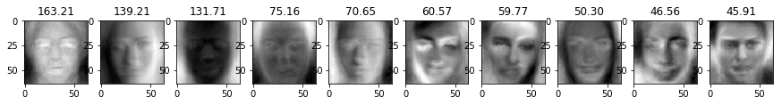
1 | # Reconstruct data with principal components |
2 | # 利用主成分进行数据重构,重构实际上就是投影的逆向操作。 |
3 | n_components = 100 # 测试不同的参数值查看对重构的影响 |
4 | X_proj = pca.transform(X_train, n_components) |
5 | X_rec = pca.reconstruct(X_proj) |
6 | |
7 | print(X_rec.shape) |
8 | print(classes) |
9 | |
10 | # 查看重构后的脸部图像 |
11 | samples_per_class = 10 |
12 | for y, cls in enumerate(classes): |
13 | idxs = np.flatnonzero(y_train == y) |
14 | idxs = np.random.choice(idxs, samples_per_class, replace=False) |
15 | for i, idx in enumerate(idxs): |
16 | plt_idx = i * num_classes + y + 1 |
17 | plt.subplot(samples_per_class, num_classes, plt_idx) |
18 | plt.imshow((X_rec[idx]).reshape((64, 64))) |
19 | plt.axis('off') |
20 | if i == 0: |
21 | plt.title(y) |
22 | plt.show() |
1 | (800, 4096) |
2 | ['angelina jolie', 'anne hathaway', 'barack obama', 'brad pitt', 'cristiano ronaldo', 'emma watson', 'george clooney', 'hillary clinton', 'jennifer aniston', 'johnny depp', 'justin timberlake', 'leonardo dicaprio', 'natalie portman', 'nicole kidman', 'scarlett johansson', 'tom cruise'] |
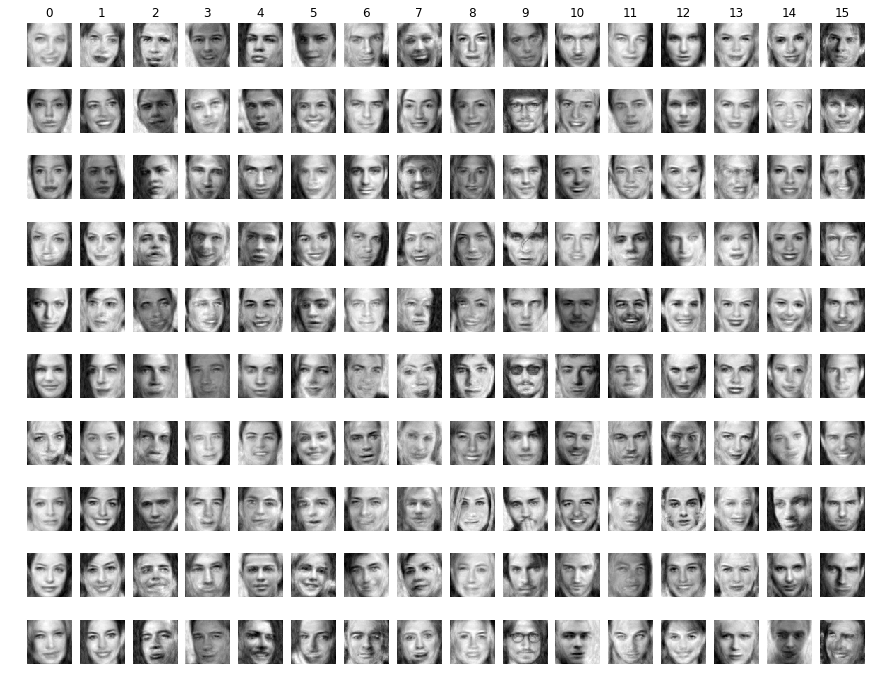
100个主成分能够分清男女了,200个主成分大概能够分清是哪个人了。
Written Question 1
Question: Consider a dataset of N face images, each with shape (h,w). Then, we need O(Nhw) of memory to store the data. Suppose we perform dimensionality reduction on the dataset with p principal components, and use the components as bases to represent images. Calculate how much memory we need to store the images and the matrix used to get back to the original space.
Said in another way, how much memory does storing the compressed images and the uncompresser cost.
- 降维后的图像维度为
X_proj.shape = (N, n_components),所以实际压缩的图像占用空间即为O(Np)- 为了实现压缩和复原的其他资源(姑且称之为解压器),需要保存的变量包括
self.W_pca和self.mean,实际上内存大头就是样本的所有主成分表,所以解压器占用的内存空间为O(pD) = O(phw)
Reconstruction error and captured variance
We can plot the reconstruction error with respect to the dimension of the projected space.
The reconstruction gets better with more components.
We can see in the plot that the inflexion point is around dimension 200 or 300. This means that using this number of components is a good compromise between good reconstruction and low dimension.
1 | # Plot reconstruction errors for different k |
2 | # 绘制出不同主成分数目对应的重构误差 |
3 | N = X_train.shape[0] |
4 | d = X_train.shape[1] |
5 | |
6 | ns = range(1, d, 20) |
7 | errors = [] |
8 | |
9 | for n in ns: |
10 | X_proj = pca.transform(X_train, n) |
11 | X_rec = pca.reconstruct(X_proj) |
12 | |
13 | # Compute reconstruction error |
14 | error = np.mean((X_rec - X_train) ** 2) |
15 | errors.append(error) |
16 | |
17 | plt.plot(ns, errors) |
18 | plt.xlabel('Number of Components') |
19 | plt.ylabel('Reconstruction Error') |
20 | plt.show() |
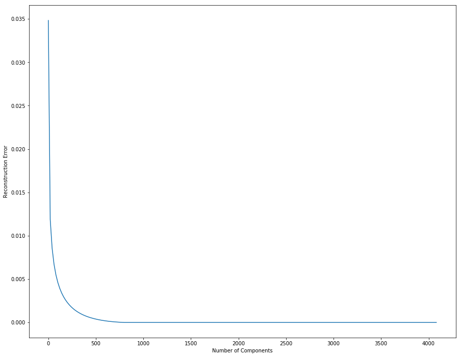
从上面这幅图可以获取到的有用信息就是:
- 1000以内,误差随着主成分数目增加而减小
- 大概在200-400间,出现了下降速率的拐角,此处可以来个权衡,因为主成分数目并不是越多越好,它影响了运行的效率。选择拐角处的值,既能保证误差率较低,还能兼顾计算时间。
We can do the same process to see how much variance is captured by the projection.
Again, we see that the inflexion point is around 200 or 300 dimensions.
同样,方差的拐点也在200-400之间
1 | # Plot captured variance |
2 | ns = range(1, d, 100) |
3 | var_cap = [] |
4 | |
5 | for n in ns: |
6 | var_cap.append(np.sum(s[:n] ** 2)/np.sum(s ** 2)) |
7 | |
8 | plt.plot(ns, var_cap) |
9 | plt.xlabel('Number of Components') |
10 | plt.ylabel('Variance Captured') |
11 | plt.show() |
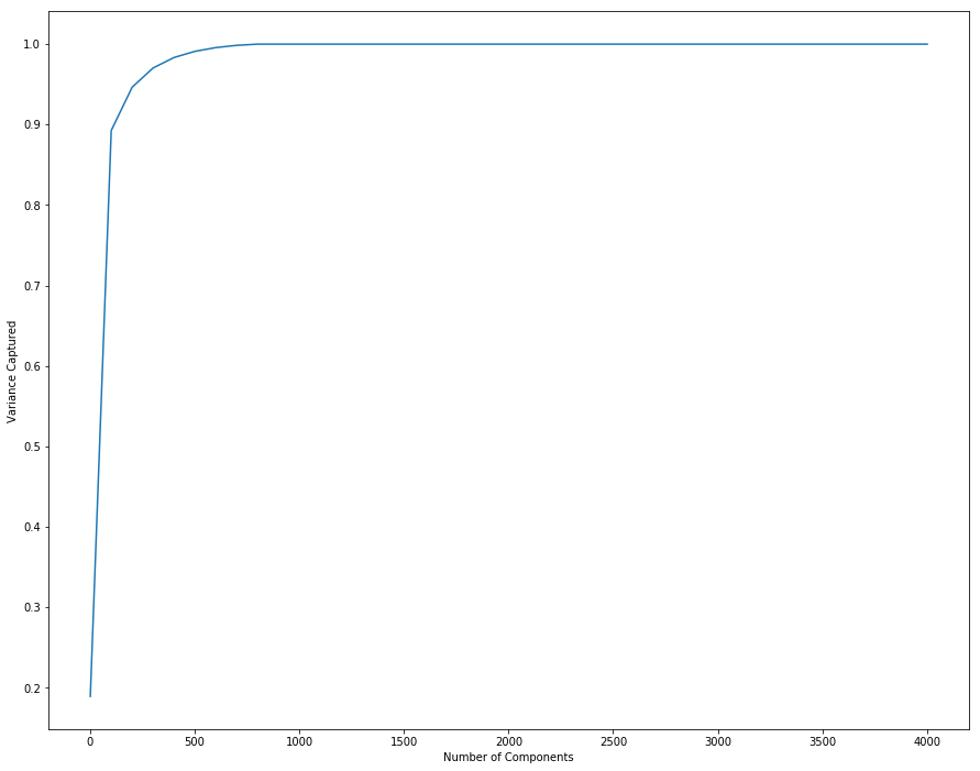
kNN with PCA
Performing kNN on raw features (the pixels of the image) does not yield very good results.
Computing the distance between images in the image space is not a very good metric for actual proximity of images.
For instance, an image of person A with a dark background will be close to an image of B with a dark background, although these people are not the same.
Using a technique like PCA can help discover the real interesting features and perform kNN on them could give better accuracy.
However, we observe here that PCA doesn’t really help to disentangle the features and obtain useful distance metrics between the different classes. We basically obtain the same performance as with raw features.
上面这段话讲的挺好,直接使用原始的特征(即图像的像素)并不能表现的很好,因为在计算图像之间的距离时,两个不同物体具有相同的黑色背景时,背景明显在计算上减小了两者之间的距离,虽然我们要判断的是前景的类别。
使用PCA能够得到有趣的特征,能够使kNN能够达到更高的准确率。
但是,在这里,PCA并不能在不同类别里区分开特征,获取到有用的距离。这里看起来和使用像素是一样的效果。
1 | num_test = X_test.shape[0] |
2 | |
3 | # We computed the best k and n for you |
4 | best_k = 20 |
5 | best_n = 100 |
6 | |
7 | |
8 | # PCA |
9 | pca = PCA() |
10 | pca.fit(X_train) |
11 | X_proj = pca.transform(X_train, best_n) |
12 | X_test_proj = pca.transform(X_test, best_n) |
13 | |
14 | # kNN |
15 | dists = compute_distances(X_test_proj, X_proj) |
16 | y_test_pred = predict_labels(dists, y_train, k=best_k) |
17 | |
18 | # Compute and display the accuracy |
19 | num_correct = np.sum(y_test_pred == y_test) |
20 | accuracy = float(num_correct) / num_test |
21 | print('Got %d / %d correct => accuracy: %f' % (num_correct, num_test, accuracy)) |
1 | Got 45 / 160 correct => accuracy: 0.281250 |
PCA有用,但就涨了这么点准确率。
因为,在这里,PCA并不能在不同类别里区分开特征,获取到有用的距离。这里看起来和使用像素是一样的效果。
Fisherface: Linear Discriminant Analysis
LDA is a linear transformation method like PCA, but with a different goal.
The main difference is that LDA takes information from the labels of the examples to maximize the separation of the different classes in the transformed space.
Therefore, LDA is not totally unsupervised since it requires labels. PCA is fully unsupervised.
In summary:
- PCA perserves maximum variance in the projected space.
- LDA preserves discrimination between classes in the project space. We want to maximize scatter between classes and minimize scatter intra class.
LDA和PCA的区别
LDA的主旨就是从标签中获取信息,在转换的目标空间最大化不同种类之间的隔离。
1 | from features import LDA |
2 | lda = LDA() |
Dimensionality Reduction via PCA
To apply LDA, we need D<N. Since in our dataset, N=800 and D=4096, we first need to reduce the number of dimensions of the images using PCA.
More information at: http://www.scholarpedia.org/article/Fisherfaces
通过PCA实现维度的缩减
这里提到数据特征维度要比样本数少,所以需要进行一步特征的维度缩减,就直接拿PCA做降维好了。
1 | N = X_train.shape[0] |
2 | c = num_classes |
3 | |
4 | pca = PCA() |
5 | pca.fit(X_train) |
6 | X_train_pca = pca.transform(X_train, N-c) |
7 | X_test_pca = pca.transform(X_test, N-c) |
Scatter matrices
We first need to compute the within-class scatter matrix:
where is the scatter of class .
We then need to compute the between-class scatter matrix:
where is the number of examples in class .
散点图矩阵
上面的公式偏向结论的,具体的推导在Lecture13 的PPT 第42页开始。
1 | # Compute within-class scatter matrix |
2 | # 计算类内散点图矩阵 |
3 | S_W = lda._within_class_scatter(X_train_pca, y_train) |
4 | print(S_W.shape) |
1 | (784, 784) |
1 | # Compute between-class scatter matrix |
2 | # 计算类间散点图矩阵 |
3 | S_B = lda._between_class_scatter(X_train_pca, y_train) |
4 | print(S_B.shape) |
1 | (784, 784) |
Solving generalized Eigenvalue problem
Implement methods fit and transform of the LDA class.
根据Lecture 第55页,最终将优化问题泛化为了一个求特征值的问题。编程时直接使用线性代数库求解特征值即可。
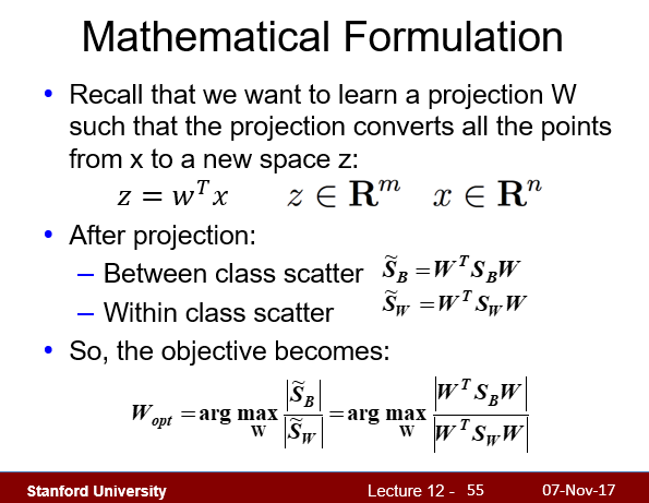
1 | lda.fit(X_train_pca, y_train) |
1 | # Dimensionality reduction by projecting the data onto |
2 | # lower dimensional subspace spanned by k principal components |
3 | # 通过K个主成分,将数据投射到低维的子空间上来实现维度缩减 |
4 | # 这个实现方式其实跟PCA应该是一样的 |
5 | n_components = 2 |
6 | X_proj = lda.transform(X_train_pca, n_components) |
7 | |
8 | X_test_proj = lda.transform(X_test_pca, n_components) |
9 | |
10 | # Plot the top two principal components on the training set |
11 | for y in np.unique(y_train): |
12 | plt.scatter(X_proj[y_train==y, 0], X_proj[y_train==y, 1], label=classes[y]) |
13 | |
14 | plt.xlabel('1st component') |
15 | plt.ylabel('2nd component') |
16 | plt.legend() |
17 | plt.title("Training set") |
18 | plt.show() |
19 | |
20 | # Plot the top two principal components on the test set |
21 | for y in np.unique(y_test): |
22 | plt.scatter(X_test_proj[y_test==y, 0], X_test_proj[y_test==y,1], label=classes[y]) |
23 | |
24 | plt.xlabel('1st component') |
25 | plt.ylabel('2nd component') |
26 | plt.legend() |
27 | plt.title("Test set") |
28 | plt.show() |
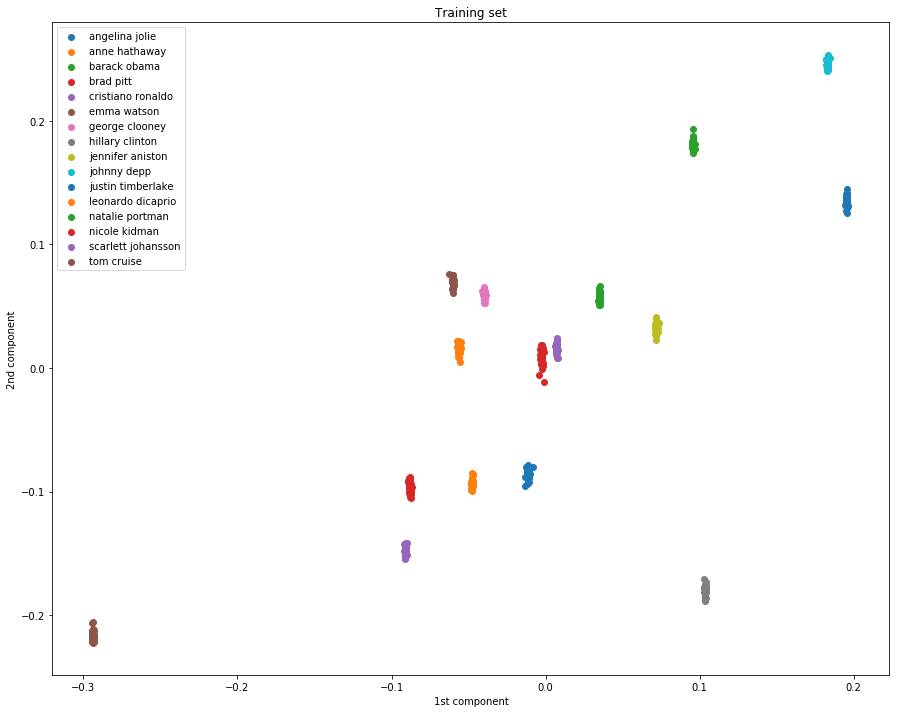
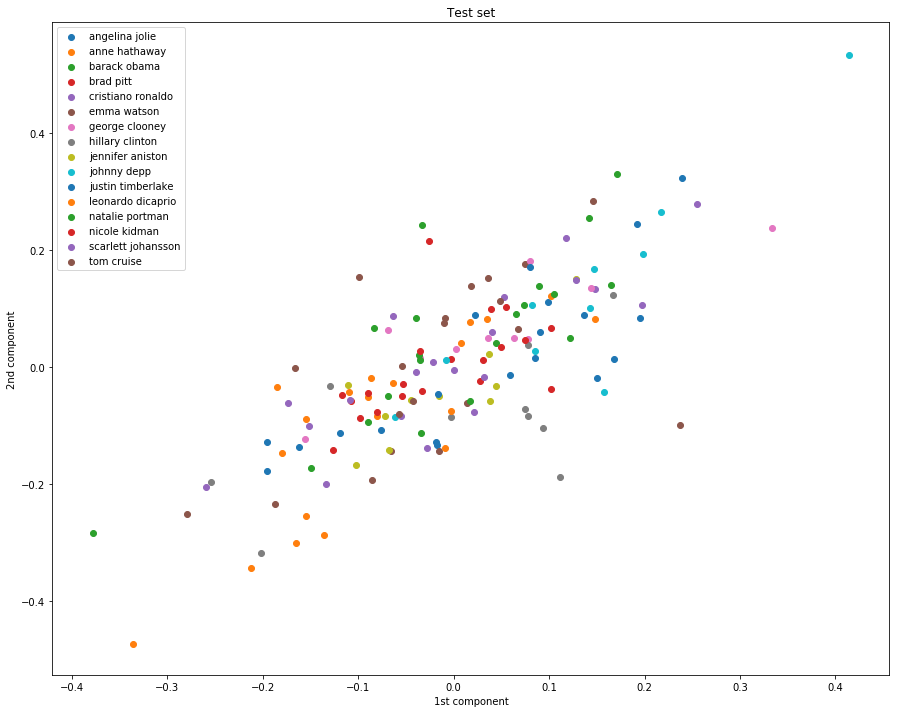
第一幅图的效果好是因为已经fit过了,即进行过了训练。
第二幅图的效果不好,泛化能力明显不行。
实现维度缩减的最后一步,投射到子空间的方式和PCA是一样的,
那么PCA和LDA唯一的不同就是寻找主成分的理念不同了,
PCA强调的是在实现维度缩减的同时最大化保留的信息量
LDA强调的则是最小化类内的区别,最大化类间的区别
kNN with LDA
Thanks to having the information from the labels, LDA gives a discriminant space where the classes are far apart from each other.
This should help kNN a lot, as the job should just be to find the obvious 10 clusters.
However, as we’ve seen in the previous plot (section 4.3), the training data gets clustered pretty well, but the test data isn’t as nicely clustered as the training data (overfitting?).
Perform cross validation following the code below (you can change the values of k_choices and n_choices to search). Using the best result from cross validation, obtain the test accuracy.
LDA具有最大化类间差距最小化类内差距的功效,所以在分类问题能够有很大帮助
Object-Detection
- 实现人脸检测
- 使用Hog表征和滑窗法进行人脸检测
- 使用图像金字塔对尺度问题进行改进
- 使用DPM(可变形组件模型)进行人脸检测
In this homework, we will implement a simplified version of object detection process. Note that the tests on the notebook are not comprehensive, autograder will contain more tests.
1 | from __future__ import print_function |
2 | import random |
3 | import numpy as np |
4 | import matplotlib.pyplot as plt |
5 | import matplotlib.patches as patches |
6 | from skimage import io |
7 | from skimage.feature import hog |
8 | from skimage import data, color, exposure |
9 | from skimage.transform import rescale, resize, downscale_local_mean |
10 | import glob, os |
11 | import fnmatch |
12 | import time |
13 | import math |
14 | |
15 | import warnings |
16 | warnings.filterwarnings('ignore') |
17 | |
18 | from detection import * |
19 | from util import * |
20 | |
21 | # This code is to make matplotlib figures appear inline in the |
22 | # notebook rather than in a new window. |
23 | %matplotlib inline |
24 | plt.rcParams['figure.figsize'] = (10.0, 8.0) # set default size of plots |
25 | plt.rcParams['image.interpolation'] = 'nearest' |
26 | plt.rcParams['image.cmap'] = 'gray' |
27 | |
28 | # Some more magic so that the notebook will reload external python modules; |
29 | # see http://stackoverflow.com/questions/1907993/autoreload-of-modules-in-ipython |
30 | %load_ext autoreload |
31 | %autoreload 2 |
32 | %reload_ext autoreload |
Hog Representation
In this section, we will compute the average hog representation of human faces.
There are 31 aligned face images provided in the \face folder. They are all aligned and have the same size. We will get an average face from these images and compute a hog feature representation for the averaged face.
Use the hog function provided by skimage library, and implement a hog representation of objects.
Implement hog_feature function in detection.py
Hog表征
这里要计算人脸的平均hog表征。可以直接调用skimage包中feature模块内的hog函数进行hog特征的提取。
1 | image_paths = fnmatch.filter(os.listdir('./face'), '*.jpg') |
2 | list.sort(image_paths) |
3 | n = len(image_paths) |
4 | face_shape = io.imread('./face/'+image_paths[0], as_grey=True).shape |
5 | avg_face= np.zeros((face_shape)) |
6 | for i,image_path in enumerate(image_paths): |
7 | image = io.imread('./face/'+image_path, as_grey=True) |
8 | avg_face = np.asarray(image)+np.asarray(avg_face) |
9 | avg_face = avg_face/n |
10 | |
11 | (face_feature, face_hog) = hog_feature(avg_face) |
12 | |
13 | plt.subplot(1,2,1) |
14 | plt.imshow(avg_face) |
15 | plt.axis('off') |
16 | plt.title('average face image') |
17 | |
18 | plt.subplot(1,2,2) |
19 | plt.imshow(face_hog) |
20 | plt.title('hog representation of face') |
21 | plt.axis('off') |
22 | |
23 | plt.show() |
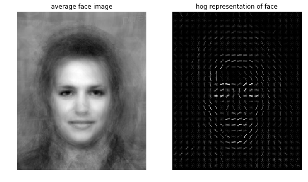
Sliding Window
Implement sliding_window function to have windows slide across an image with a specific window size. The window slides through the image and check if an object is detected with a high score at every location. These scores will generate a response map and you will be able to find the location of the window with the highest hog score.
滑窗法
滑窗法就是定义一个窗体对象(匹配对象),遍历图像中的图像块,计算卷积响应(此处对两者Hog特征序列进行内积计算),输出值最高的地方就是图像中与匹配对象最相似的地方。
1 | image_path = 'image_0001.jpg' |
2 | |
3 | image = io.imread(image_path, as_grey=True) |
4 | image = rescale(image, 0.8) |
5 | |
6 | (hogFeature, hogImage) = hog_feature(image) |
7 | |
8 | (winH, winW) = face_shape |
9 | (score, r, c, response_map) = sliding_window(image, face_feature, stepSize=30, windowSize=face_shape) |
10 | crop = image[r:r+winH, c:c+winW] |
11 | |
12 | fig,ax = plt.subplots(1) |
13 | ax.imshow(image) |
14 | rect = patches.Rectangle((c,r),winW,winH,linewidth=1,edgecolor='r',facecolor='none') |
15 | ax.add_patch(rect) |
16 | plt.show() |
17 | |
18 | plt.imshow(response_map,cmap='viridis', interpolation='nearest') |
19 | plt.title('sliding window') |
20 | plt.show() |
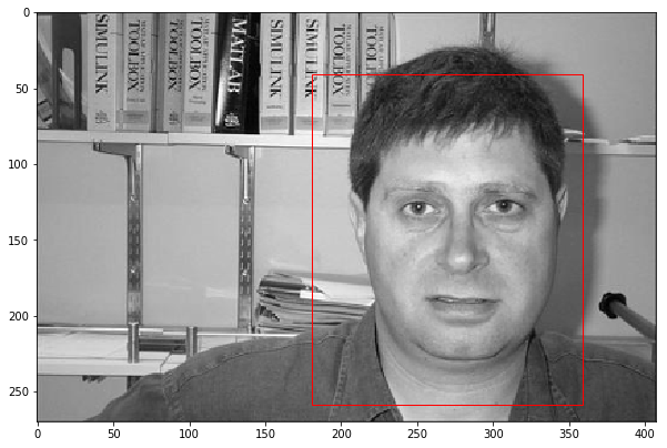
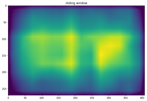
Sliding window successfully found the human face in the above example. However, in the cell below, we are only changing the scale of the image, and you can see that sliding window does not work once the scale of the image is changed.
上面的图像能够检测到人脸的正确区域,但是下面这张图却出现了错误。说明滑窗这种方法对于图像的尺度十分敏感。
1 | image_path = 'image_0001.jpg' |
2 | image = io.imread(image_path, as_grey=True) |
3 | image = rescale(image, 1.0) |
4 | |
5 | |
6 | (winH, winW) = face_shape |
7 | (score, r, c, max_response_map) = sliding_window(image, face_feature, stepSize=30, windowSize=face_shape) |
8 | |
9 | crop = image[r:r+winH, c:c+winW] |
10 | |
11 | fig,ax = plt.subplots(1) |
12 | ax.imshow(image) |
13 | rect = patches.Rectangle((c,r),winW,winH,linewidth=1,edgecolor='r',facecolor='none') |
14 | ax.add_patch(rect) |
15 | plt.show() |
16 | |
17 | plt.imshow(max_response_map,cmap='viridis', interpolation='nearest') |
18 | plt.title('sliding window') |
19 | plt.axis('off') |
20 | plt.show() |
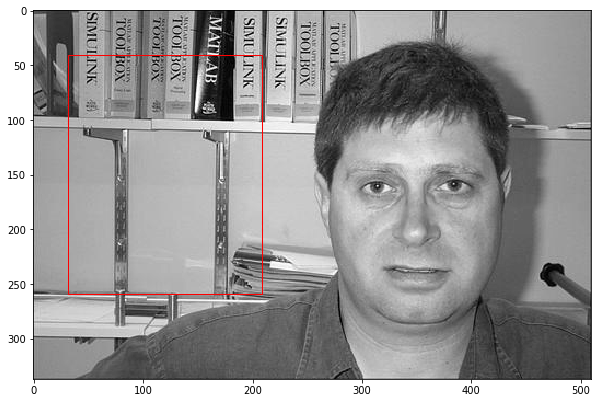
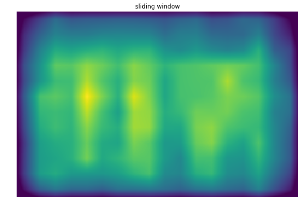
Image Pyramids
In order to make sliding window work for different scales of images, you need to implement image pyramids where you resize the image to different scales and run the sliding window method on each resized image. This way you scale the objects and can detect both small and large objects.
针对上面的问题,需要采用图像金字塔的方案来进行匹配。
代码中直接是使用resize函数,生成了不同尺度的图像,具体的图像金字塔实现可以看博客,上采样和下采样是利用高斯滤波器和插值滤波器实现的。
Image Pyramid
Implement pyramid function in detection.py, this will create pyramid of images at different scales. Run the following code, and you will see the shape of the original image gets smaller until it reaches a minimum size.
1 | image_path = 'image_0001.jpg' |
2 | |
3 | image = io.imread(image_path, as_grey=True) |
4 | image = rescale(image, 1.2) |
5 | |
6 | images = pyramid(image, scale = 0.9) |
7 | sum_r = 0 |
8 | sum_c = 0 |
9 | for i,result in enumerate(images): |
10 | (scale, image) = result |
11 | if (i==0): |
12 | sum_c = image.shape[1] |
13 | sum_r+=image.shape[0] |
14 | |
15 | composite_image = np.zeros((sum_r, sum_c)) |
16 | |
17 | pointer = 0 |
18 | for i, result in enumerate(images): |
19 | (scale, image) = result |
20 | composite_image[pointer:pointer+image.shape[0], :image.shape[1]] = image |
21 | pointer+= image.shape[0] |
22 | |
23 | plt.imshow(composite_image) |
24 | plt.axis('off') |
25 | plt.title('image pyramid') |
26 | plt.show() |
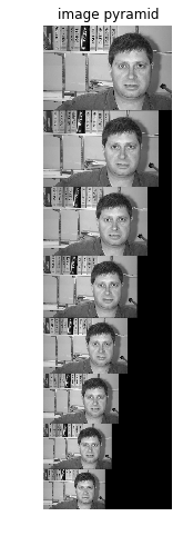
Pyramid Score
After getting the image pyramid, we will run sliding window on all the images to find a place that gets the highest score. Implement pyramid_score function in detection.py. It will return the highest score and its related information in the image pyramids.
1 | image_path = 'image_0001.jpg' |
2 | |
3 | image = io.imread(image_path, as_grey=True) |
4 | image = rescale(image, 1.4) |
5 | |
6 | (winH, winW) = face_shape |
7 | max_score, maxr, maxc, max_scale, max_response_map = pyramid_score \ |
8 | (image, face_feature, face_shape, stepSize = 30, scale=0.8) |
9 | |
10 | fig,ax = plt.subplots(1) |
11 | ax.imshow(rescale(image, max_scale)) |
12 | rect = patches.Rectangle((maxc,maxr),winW,winH,linewidth=3,edgecolor='r',facecolor='none') |
13 | ax.add_patch(rect) |
14 | plt.show() |
15 | |
16 | plt.imshow(max_response_map, cmap='viridis', interpolation='nearest') |
17 | plt.axis('off') |
18 | plt.show() |
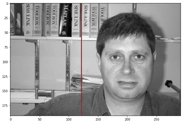
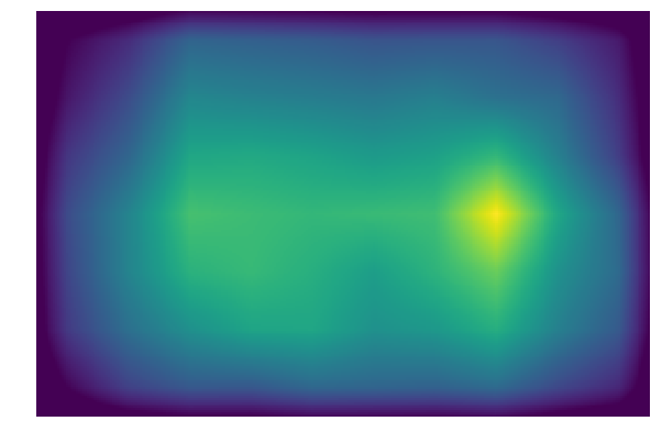
From the above example, we can see that image pyramid has fixed the problem of scaling. Then in the example below, we will try another image and implement deformable part model.
通过调整image = rescale(image, 1.2)中的缩放比例,可以看到,图像金字塔的方案还是能解决掉上一步中尺度引起的问题的。
1 | image_path = 'image_0338.jpg' |
2 | image = io.imread(image_path, as_grey=True) |
3 | image = rescale(image, 1.0) |
4 | |
5 | (winH, winW) = face_shape |
6 | |
7 | max_score, maxr, maxc, max_scale, max_response_map = pyramid_score \ |
8 | (image, face_feature, face_shape, stepSize = 30, scale=0.8) |
9 | |
10 | fig,ax = plt.subplots(1) |
11 | ax.imshow(rescale(image, max_scale)) |
12 | rect = patches.Rectangle((maxc,maxr),winW,winH,linewidth=1,edgecolor='r',facecolor='none') |
13 | ax.add_patch(rect) |
14 | plt.show() |
15 | |
16 | plt.imshow(max_response_map,cmap='viridis', interpolation='nearest') |
17 | plt.axis('off') |
18 | plt.show() |
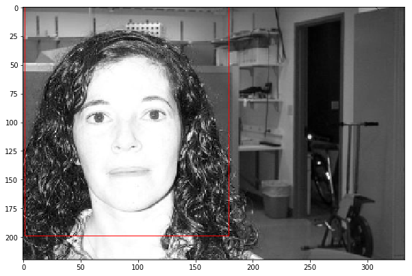

Deformable Parts Detection
In order to solve the problem above, you will implement deformable parts model in this section, and apply it on human faces.
The first step is to get a detector for each part of the face, including left eye, right eye, nose and mouth.
For example for the left eye, we have provided the groundtruth location of left eyes for each image in the \face directory. This is stored in the lefteyes array with shape (n,2), each row is the (r,c) location of the center of left eye. You will then find the average hog representation of the left eyes in the images.
下面四块分别是左眼、右眼、鼻子和眼镜的检测器。
代码是作业本身就提供了的,不过可以仔细研究一下具体实现。
Run through the following code to get a detector for left eyes.
1 | image_paths = fnmatch.filter(os.listdir('./face'), '*.jpg') |
2 | |
3 | parts = read_facial_labels(image_paths) |
4 | lefteyes, righteyes, noses, mouths = parts |
5 | |
6 | # Typical shape for left eye |
7 | lefteye_h = 10 |
8 | lefteye_w = 20 |
9 | |
10 | lefteye_shape = (lefteye_h, lefteye_w) |
11 | |
12 | avg_lefteye = get_detector(lefteye_h, lefteye_w, lefteyes, image_paths) |
13 | (lefteye_feature, lefteye_hog) = hog_feature(avg_lefteye, pixel_per_cell=2) |
14 | |
15 | plt.subplot(1,3,1) |
16 | plt.imshow(avg_lefteye) |
17 | plt.axis('off') |
18 | plt.title('average left eye image') |
19 | |
20 | plt.subplot(1,3,2) |
21 | plt.imshow(lefteye_hog) |
22 | plt.axis('off') |
23 | plt.title('average hog image') |
24 | plt.show() |
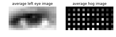
Run through the following code to get a detector for right eye.
1 | righteye_h = 10 |
2 | righteye_w = 20 |
3 | |
4 | righteye_shape = (righteye_h, righteye_w) |
5 | |
6 | avg_righteye = get_detector(righteye_h, righteye_w, righteyes, image_paths) |
7 | |
8 | (righteye_feature, righteye_hog) = hog_feature(avg_righteye, pixel_per_cell=2) |
9 | |
10 | plt.subplot(1,3,1) |
11 | plt.imshow(avg_righteye) |
12 | plt.axis('off') |
13 | plt.title('average right eye image') |
14 | |
15 | plt.subplot(1,3,2) |
16 | plt.imshow(righteye_hog) |
17 | plt.axis('off') |
18 | plt.title('average hog image') |
19 | plt.show() |
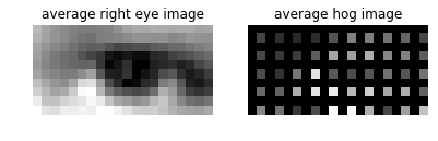
Run through the following code to get a detector for nose.
1 | nose_h = 30 |
2 | nose_w = 26 |
3 | |
4 | nose_shape = (nose_h, nose_w) |
5 | |
6 | avg_nose = get_detector(nose_h, nose_w, noses, image_paths) |
7 | |
8 | (nose_feature, nose_hog) = hog_feature(avg_nose, pixel_per_cell=2) |
9 | |
10 | plt.subplot(1,3,1) |
11 | plt.imshow(avg_nose) |
12 | plt.axis('off') |
13 | plt.title('average nose image') |
14 | |
15 | plt.subplot(1,3,2) |
16 | plt.imshow(nose_hog) |
17 | plt.axis('off') |
18 | plt.title('average hog image') |
19 | plt.show() |
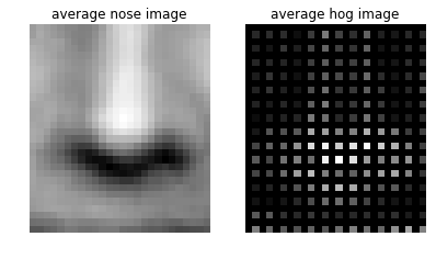
Run through the following code to get a detector for mouth
1 | mouth_h = 20 |
2 | mouth_w = 36 |
3 | |
4 | mouth_shape = (mouth_h, mouth_w) |
5 | |
6 | avg_mouth = get_detector(mouth_h, mouth_w, mouths, image_paths) |
7 | |
8 | (mouth_feature, mouth_hog) = hog_feature(avg_mouth, pixel_per_cell=2) |
9 | |
10 | detectors_list = [lefteye_feature, righteye_feature, nose_feature, mouth_feature] |
11 | |
12 | plt.subplot(1,3,1) |
13 | plt.imshow(avg_mouth) |
14 | plt.axis('off') |
15 | plt.title('average mouth image') |
16 | |
17 | plt.subplot(1,3,2) |
18 | plt.imshow(mouth_hog) |
19 | plt.axis('off') |
20 | plt.title('average hog image') |
21 | plt.show() |

Human Parts Location
Implement compute_displacement to get an average shift vector mu and standard deviation sigma for each part of the face. The vector mu is the distance from the main center, i.e the center of the face, to the center of the part.
找到各个部位的位置
这里计算的是相对位置,即各个组件的中心与脸部中心的距离。
1 | # test for compute_displacement |
2 | test_array = np.array([[0,1],[1,2],[2,3],[3,4]]) |
3 | test_shape = (6,6) |
4 | mu, std = compute_displacement(test_array, test_shape) |
5 | assert(np.all(mu == [1,0])) |
6 | assert(np.sum(std-[ 1.11803399, 1.11803399])<1e-5) |
7 | print("Your implementation is correct!") |
1 | Your implementation is correct! |
1 | lefteye_mu, lefteye_std = compute_displacement(lefteyes, face_shape) |
2 | righteye_mu, righteye_std = compute_displacement(righteyes, face_shape) |
3 | nose_mu, nose_std = compute_displacement(noses, face_shape) |
4 | mouth_mu, mouth_std = compute_displacement(mouths, face_shape) |
After getting the shift vectors, we can run our detector on a test image. We will first run the following code to detect each part of left eye, right eye, nose and mouth in the image. You will see a response map for each of them.
分别使用脸部和各个组件的检测器,对整张图像进行匹配计算,得到每个组件的响应图。
1 | image_path = 'image_0338.jpg' |
2 | image = io.imread(image_path, as_grey=True) |
3 | image = rescale(image, 1.0) |
4 | |
5 | (face_H, face_W) = face_shape |
6 | max_score, face_r, face_c, face_scale, face_response_map = pyramid_score\ |
7 | (image, face_feature, face_shape,stepSize = 30, scale=0.8) |
8 | |
9 | plt.imshow(face_response_map, cmap='viridis', interpolation='nearest') |
10 | plt.axis('off') |
11 | plt.show() |
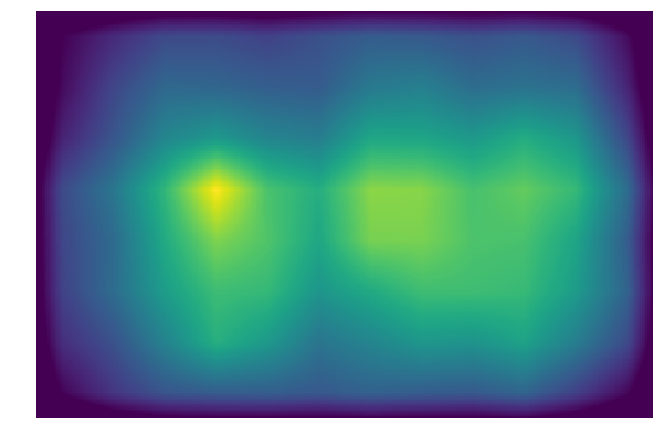
1 | max_score, lefteye_r, lefteye_c, lefteye_scale, lefteye_response_map = \ |
2 | pyramid_score(image, lefteye_feature,lefteye_shape, stepSize = 20,scale=0.9, pixel_per_cell = 2) |
3 | |
4 | lefteye_response_map = resize(lefteye_response_map, face_response_map.shape) |
5 | |
6 | plt.imshow(lefteye_response_map,cmap='viridis', interpolation='nearest') |
7 | plt.axis('off') |
8 | plt.show() |
1 | max_score, righteye_r, righteye_c, righteye_scale, righteye_response_map = \ |
2 | pyramid_score (image, righteye_feature, righteye_shape, stepSize = 20,scale=0.9, pixel_per_cell=2) |
3 | |
4 | righteye_response_map = resize(righteye_response_map, face_response_map.shape) |
5 | |
6 | plt.imshow(righteye_response_map,cmap='viridis', interpolation='nearest') |
7 | plt.axis('off') |
8 | plt.show() |
1 | max_score, nose_r, nose_c, nose_scale, nose_response_map = \ |
2 | pyramid_score (image, nose_feature, nose_shape, stepSize = 20,scale=0.9, pixel_per_cell = 2) |
3 | |
4 | nose_response_map = resize(nose_response_map, face_response_map.shape) |
5 | |
6 | plt.imshow(nose_response_map,cmap='viridis', interpolation='nearest') |
7 | plt.axis('off') |
8 | plt.show() |
1 | max_score, mouth_r, mouth_c, mouth_scale, mouth_response_map =\ |
2 | pyramid_score (image, mouth_feature, mouth_shape, stepSize = 20,scale=0.9, pixel_per_cell = 2) |
3 | |
4 | mouth_response_map = resize(mouth_response_map, face_response_map.shape) |
5 | plt.imshow(mouth_response_map,cmap='viridis', interpolation='nearest') |
6 | plt.axis('off') |
7 | plt.show() |
After getting the response maps for each part of the face, we will shift these maps so that they all have the same center as the face. We have calculated the shift vector mu in compute_displacement, so we are shifting based on vector mu. Implement shift_heatmap function in detection.py.
得到各个组件的响应图之后,移动这些响应图,使得它们的中心和脸部的中心相同,方便求和。
1 | face_heatmap_shifted = shift_heatmap(face_response_map, [0,0]) |
2 | |
3 | lefteye_heatmap_shifted = shift_heatmap(lefteye_response_map, lefteye_mu) |
4 | righteye_heatmap_shifted = shift_heatmap(righteye_response_map, righteye_mu) |
5 | nose_heatmap_shifted = shift_heatmap(nose_response_map, nose_mu) |
6 | mouth_heatmap_shifted = shift_heatmap(mouth_response_map, mouth_mu) |
7 | |
8 | f, axarr = plt.subplots(2,2) |
9 | axarr[0,0].axis('off') |
10 | axarr[0,1].axis('off') |
11 | axarr[1,0].axis('off') |
12 | axarr[1,1].axis('off') |
13 | axarr[0,0].imshow(lefteye_heatmap_shifted,cmap='viridis', interpolation='nearest') |
14 | axarr[0,1].imshow(righteye_heatmap_shifted,cmap='viridis', interpolation='nearest') |
15 | axarr[1,0].imshow(nose_heatmap_shifted,cmap='viridis', interpolation='nearest') |
16 | axarr[1,1].imshow(mouth_heatmap_shifted,cmap='viridis', interpolation='nearest') |
17 | plt.show() |
Gaussian Filter
In this part, apply gaussian filter convolution to each heatmap. Blur by kernel of standard deviation sigma, and then add the heatmaps of the parts with the heatmap of the face. On the combined heatmap, find the maximum value and its location. You can use function provided by skimage to implement gaussian_heatmap.
这个部分呢,就是将之前的各个组件的响应图给叠加起来,然后判断图像区域内哪个点的响应最大,则该处判断为人脸区域。
1 | heatmap_face= face_heatmap_shifted |
2 | |
3 | # 这里将各个组件构建数组,传入 |
4 | heatmaps = [lefteye_heatmap_shifted, |
5 | righteye_heatmap_shifted, |
6 | nose_heatmap_shifted, |
7 | mouth_heatmap_shifted] |
8 | sigmas = [lefteye_std, righteye_std, nose_std, mouth_std] |
9 | |
10 | heatmap, i , j = gaussian_heatmap(heatmap_face, heatmaps, sigmas) |
11 | |
12 | fig,ax = plt.subplots(1) |
13 | rect = patches.Rectangle((j-winW//2, i-winH//2),winW,winH,linewidth=1,edgecolor='r',facecolor='none') |
14 | ax.add_patch(rect) |
15 | |
16 | plt.imshow(heatmap,cmap='viridis', interpolation='nearest') |
17 | plt.axis('off') |
18 | plt.show() |
19 | |
20 | fig,ax = plt.subplots(1) |
21 | rect = patches.Rectangle((j-winW//2, i-winH//2),winW,winH,linewidth=1,edgecolor='r',facecolor='none') |
22 | ax.add_patch(rect) |
23 | |
24 | plt.imshow(resize(image, heatmap.shape)) |
25 | plt.axis('off') |
26 | plt.show() |
Result Analysis
Does your DPM work on detecting human faces? Can you think of a case where DPM may work better than the detector we had in part 3 (sliding window + image pyramid)? You can also have examples that are not faces.
DPM的原理是很能理解的,就是将各个组件的响应值累加起来,判断哪个区域拥有最高的响应值。
上图的检测出现了问题,怀疑是脸部组件的检测不咋滴。
Extra Credit
You have tried detecting one face from the image, and the next step is to extend it to detecting multiple occurences of the object. For example in the following image, how do you detect more than one face from your response map? Implement the function detect_multiple, and write code to visualize your detected faces in the cell below.
Tracking-OpticalFlow
使用光流实现目标追踪。
实现LK光流法。
使用高斯迭代法求解LK光流。
使用金字塔方法优化LK光流。
This assignment covers Lukas-Kanade tracking method. Please hand in motion.py and this notebook file to Gradescope.
这份作业是实现Lukas-Kanade光流追踪算法。
Displaying Video
We have done some cool stuff with static images in past assignemnts. Now, let’s turn our attention to videos! For this assignment, the videos are provided as time series of images. We also provide utility functions to load the image frames and visualize them as a short video clip.
Note: You may need to install video codec like FFmpeg. For Linux/Mac, you will be able to install ffmpeg using apt-get or brew. For Windows, you can find the installation instructions here.
1 | from utils import animated_frames, load_frames |
2 | frames = load_frames('images') |
3 | ani = animated_frames(frames) |
4 | HTML(ani.to_html5_video()) |
Lucas-Kanade Method for Optical Flow
Deriving optical flow equation
Optical flow methods are used to estimate motion at each pixel location in two consecutive image frames. The optical flow equation at a spatio-temporal point is given by:
where and are partial derivatives of pixel intensity , and and are flow vectors.
Let us derive the equation in order to understand what it actually means. First, we make a reasonable assumption (a.k.a. brightness constancy) that the pixel intensity of a moving point stays the same between two consecutive frames with small time difference. Consider pixel intensity of a point in the first frame . Suppose that the point has moved to after . According to the brightness constancy constraint, we can relate intensities of the point in the two frames using the following equation:
- a. Derive the optical flow equation from the brightness constancy equation. Clearly state any assumption you make during derivation.
光流公式的推导
利用灰度不变假设,我们有: $$I(x,y,t)=I(x+Δx,y+Δy,t+Δt)$$
对右边进行泰勒展开,保留一阶项,得:$$I(x+Δx,y+Δy,t+Δt)≈I(x,y,t)+I_xΔx+I_yΔy+I_tΔt$$
因为我们假设了灰度不变,所以下个时刻的灰度等于之前的灰度,从而:$$I_xΔx+I_yΔy+I_tΔt=0$$
两边除以 ,得:$$I_x\frac{\Delta x}{\Delta t} + I_y\frac{\Delta y}{\Delta t} + I_t = 0$$
其中,表示像素在x轴上的运动速度,表示像素在y轴上的运动速度,用和表示,最终得$$I_x§v_x + I_y§v_y + I_t§ = 0$$
- b. Can the optical flow equation be solved given two consecutive frames without further assumption? Which values can be computed directly given two consecutive frames? Which values cannot be computed without additional information?
不能求解。
上式中,可以经由连续的两幅图像求解,表示图像在点处方向的梯度,表示图像在点处方向的梯度,表示图像灰度对时间的变化量。
但是仍有两个未知变量和,最终得到的是一个两个变量的一次方程。
无法求解,需要引入其他约束。
Overview of Lucas-Kanade method
The Lucas–Kanade method assumes that the motion of the image contents between two frames is approximately constant within a neighborhood of the point p under consideration (spatial coherence).
Consider a neighborhood of , (e.g. 3x3 window around ). According to the optical flow equation and spatial coherence assumption, the following should be satisfied:
For every , $$I_x(p_i)v_x+I_y(p_i)v_y=−I_t(p_i)$$
These equations can be written in matrix form , where $$A = \begin{bmatrix}I_x(p_1) & I_y(p_1) \ I_x(p_2) & I_y(p_2) \ \vdots & \vdots \ I_x(p_n) & I_y(p_n) \end{bmatrix} \hspace{1em} v = \begin{bmatrix}v_x \ v_y\end{bmatrix} \hspace{1em} b = \begin{bmatrix}-I_t(p_1) \ -I_t(p_2) \ -I_t(p_n)\end{bmatrix}$$
Note that this linear system may not have solution for v as it is usually over-determined. Instead, Lucas-Kanade method estimates the flow vector by solving the least-squares problem, .
- a. What is the condition for this equation to be solvable?
- b. Reason about why Harris corners might be good features to track using Lucas-Kanade method.
Lucas-Kanade算法的思想
上一个光流公式的推导可以得知:求解光流公式需要引入其他约束,而LK光流法的约束就是,假设某一个窗口内的像素具有相同的运动。
如果是采用3x3的窗口,则会另有9个公式,此时采用最小二乘来估计最优的和即可。
问题a:方程求解的条件是什么?参见lecture17 PPT
- 可逆
- 因为噪声的存在, 不能太小
的特征值和都不能太小
- 应当是well-conditioned
不能太大(是较大的特征值)
问题b:为何Harris角点会是LK光流法追踪的好特征?参见lecture17 PPT第25页
因为是二阶矩矩阵,的特征向量和特征值与边缘的方向和强度相关。
- 较大的特征值对应的特征向量表示强度变化最快的方向
- 另外一个特征向量则与它正交
Implementation of Lucas-Kanade method
In this section, we are going to implement basic Lucas-Kanade method for feature tracking. In order to do so, we first need to find keypoints to track. Harris corner detector is commonly used to initialize the keypoints to track with Lucas-Kanade method. For this assignment, we are going to use skimage implementation of Harris corner detector.
实现基础版本LK光流
第一步需要找到关键点来进行追踪。
Lucas-Kanade方法通常是使用Harris角点检测器来进行关键点的初始化。
skimage中提供了Harris角点检测的实现。
skimage中的Harris角点检测可以参考:Programming Computer Vision with Python (学习笔记九)
1 | from skimage import filters |
2 | from skimage.feature import corner_harris, corner_peaks |
3 | |
4 | frames = load_frames('images') |
5 | |
6 | # Detect keypoints to track |
7 | |
8 | keypoints = corner_peaks(corner_harris(frames[0]), |
9 | exclude_border=5, |
10 | threshold_rel=0.01) |
11 | |
12 | # Plot kepoints |
13 | plt.figure(figsize=(15,12)) |
14 | plt.imshow(frames[0]) |
15 | plt.scatter(keypoints[:,1], keypoints[:,0], |
16 | facecolors='none', edgecolors='r') |
17 | plt.axis('off') |
18 | plt.title('Detected keypoints in the first frame') |
19 | plt.show() |
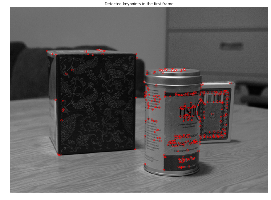
Implement function lucas_kanade in motion.py and run the code cell below. You will be able to see small arrows pointing towards the directions where keypoints are moving.
实现两帧之间的LK光流追踪
1 | from motion import lucas_kanade |
2 | |
3 | # Lucas-Kanade method for optical flow |
4 | flow_vectors = lucas_kanade(frames[0], frames[1], keypoints, window_size=5) |
5 | |
6 | # Plot flow vectors |
7 | plt.figure(figsize=(15,12)) |
8 | plt.imshow(frames[0]) |
9 | plt.axis('off') |
10 | plt.title('Optical flow vectors') |
11 | |
12 | # 用箭头标记 |
13 | for y, x, vy, vx in np.hstack((keypoints, flow_vectors)): |
14 | plt.arrow(x, y, vx, vy, head_width=5, head_length=5, color='b') |
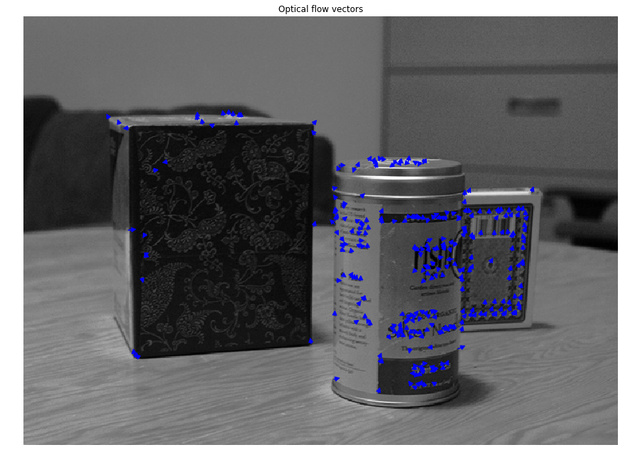
We can estimate the position of the keypoints in the next frame by adding the flow vectors to the keypoints.
通过当前帧关键点的位置和光流的方向,就可以预测下一帧中的关键点的位置
1 | # Plot tracked kepoints |
2 | new_keypoints = keypoints + flow_vectors |
3 | plt.figure(figsize=(15,12)) |
4 | plt.imshow(frames[1]) |
5 | plt.scatter(new_keypoints[:,1], new_keypoints[:,0], |
6 | facecolors='none', edgecolors='r') |
7 | plt.axis('off') |
8 | plt.title('Tracked keypoints in the second frame') |
9 | plt.show() |

上图可以看到,光流法预测的第二帧中的特征点地位置还是基本正确的。
Feature Tracking in multiple frames
Now we can use Lucas-Kanade method to track keypoints across multiple frames. The idea is simple: compute flow vectors at keypoints in -th frame, and add the flow vectors to the points to keep track of the points in -th frame. We have provided the function track_features for you. First, run the code cell below. You will notice that some of the points just drift away and are not tracked very well.
Instead of keeping these ‘bad’ tracks, we would want to somehow declare some points are ‘lost’ and just discard them. One simple way to is to compare the patches around tracked points in two subsequent frames. If the patch around a point is NOT similar to the patch around the corresponding point in the next frame, then we declare the point to be lost. Here, we are going to use mean squared error between two normalized patches as the criterion for lost tracks.
Implement compute_error in motion.py, and re-run the code cell below. You will see many of the points disappearing in later frames.
作业中已经提供了追踪连续图像帧中的特征点的功能,在track_features函数中。
其中思路就是根据初始的关键点位置和相邻两帧LK光流法得到的光流方向,计算预测后续每一帧中的关键点位置。
但是由于出现一些关键点的漂移(计算精确度以及关键点的消失),整体的追踪效果会很差。
为了去除这些“坏点” 的影响,提出了一种思路就是:判断关键点的丢失。
原理就是:判断相邻两帧关键点区域图像块的相似程度,如果不相似则判断为该点丢。它的依据就是Lucas-Kanade的假设,某一窗口内的像素具有相同的移动。
计算方式:计算两个归一化的图像块的均方差MSE,如果大于阈值,则抛弃该点。
1 | from utils import animated_scatter |
2 | from motion import track_features |
3 | |
4 | # Detect keypoints to track in the first frame |
5 | keypoints = corner_peaks(corner_harris(frames[0]), |
6 | exclude_border=5, |
7 | threshold_rel=0.01) |
8 | |
9 | trajs = track_features(frames, keypoints, |
10 | error_thresh=1.5, |
11 | optflow_fn=lucas_kanade, |
12 | window_size=5) |
13 | |
14 | ani = animated_scatter(frames,trajs) |
15 | HTML(ani.to_html5_video()) |
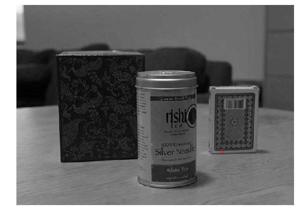
从上面的运行效果看,保留下来的关键点都能够准确的被预测到。
但是也可以看到就是,当运动幅度较大的时候,好多关键点都被丢弃了。
Pyramidal Lucas-Kanade Feature Tracker
In this section, we are going to implement a simpler version of the method described in “Pyramidal Implementation of the Lucas Kanade Feature Tracker”.
金字塔光流法
Iterative Lucas-Kanade method
One limitation of the naive Lucas-Kanade method is that it cannot track large motions between frames. You might have noticed that the resulting flow vectors (blue arrows) in the previous section are too small that the tracked keypoints are slightly off from where they should be. In order to address this problem, we can iteratively refine the estimated optical flow vectors. Below is the step-by-step description of the algorithm:
Let be a point on frame . The goal is to find flow vector such that is the corresponding point of on the next frame .
- Initialize flow vector: $$v = \begin{bmatrix}0\0\end{bmatrix}$$
- Compute spatial gradient matrix:
- for to
- Compute temporal difference:
- Compute image mismatch vector
Compute optical flow:
Update flow vector for next iteration:
- Return
Implement iterative_lucas_kanade method in motion.py and run the code cell below. You should be able to see slightly longer arrows in the visualization.
1 | from motion import iterative_lucas_kanade |
2 | |
3 | # Run iterative Lucas-Kanade method |
4 | flow_vectors = iterative_lucas_kanade(frames[0], frames[1], keypoints) |
5 | |
6 | # Plot flow vectors |
7 | plt.figure(figsize=(15,12)) |
8 | plt.imshow(frames[0]) |
9 | plt.axis('off') |
10 | plt.title('Optical flow vectors (iterative LK)') |
11 | |
12 | for y, x, vy, vx in np.hstack((keypoints, flow_vectors)): |
13 | plt.arrow(x, y, vx, vy, head_width=5, head_length=5, color='b') |
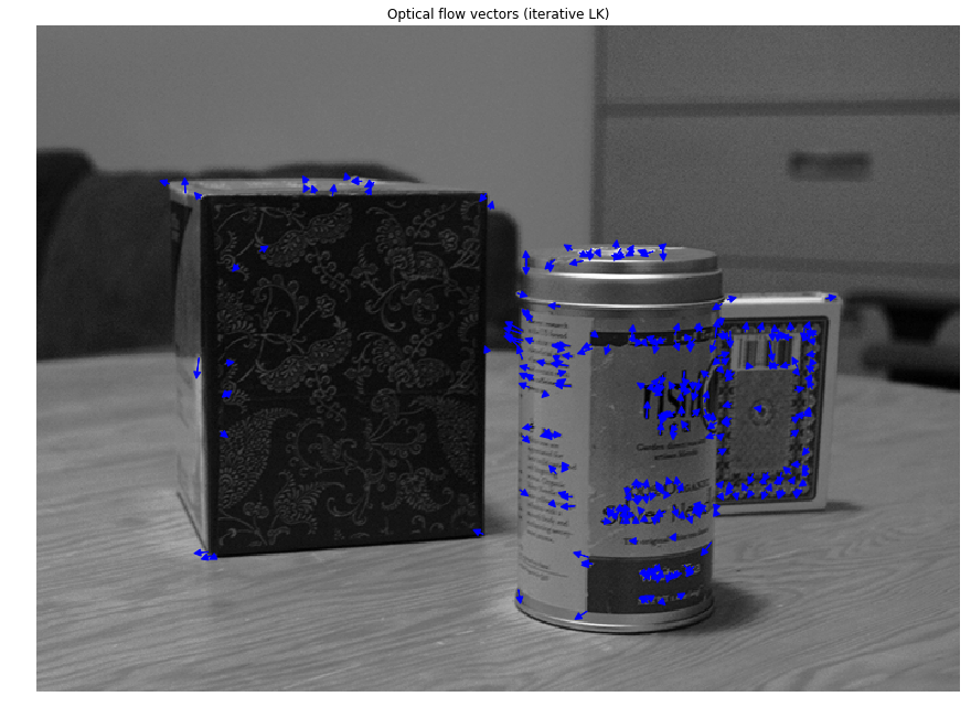
可以看到,迭代式光流法可以检测到大运动的光流。
1 | # Plot tracked kepoints |
2 | new_keypoints = keypoints + flow_vectors |
3 | plt.figure(figsize=(15,12)) |
4 | plt.imshow(frames[1]) |
5 | plt.scatter(new_keypoints[:,1], new_keypoints[:,0], |
6 | facecolors='none', edgecolors='r') |
7 | plt.axis('off') |
8 | plt.title('Tracked keypoints in the second frame (iterative LK)') |
9 | plt.show() |
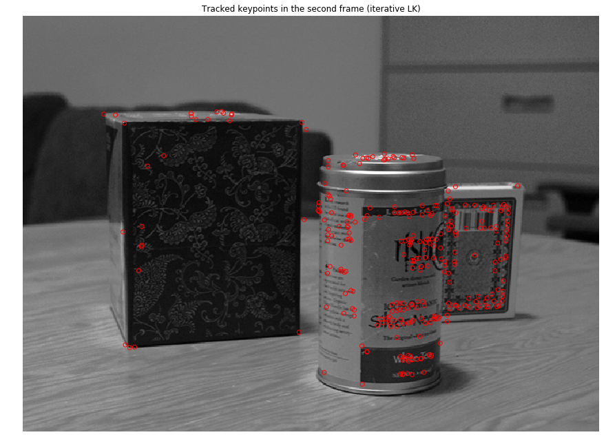
1 | # Detect keypoints to track in the first frame |
2 | keypoints = corner_peaks(corner_harris(frames[0]), |
3 | exclude_border=5, |
4 | threshold_rel=0.01) |
5 | |
6 | # Track keypoints using iterative Lucas-Kanade method |
7 | trajs = track_features(frames, keypoints, |
8 | error_thresh=1.5, |
9 | optflow_fn=iterative_lucas_kanade, |
10 | window_size=5) |
11 | ani = animated_scatter(frames,trajs) |
12 | HTML(ani.to_html5_video())todo_tracking_sample2 |
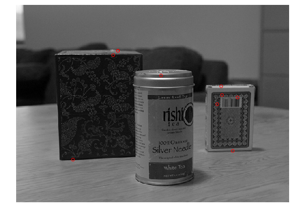
运行到最后,相比于之前LK光流,迭代式光流法追踪并保留了更多的关键点。
Coarse-to-Fine Optical Flow
The iterative method still could not track larger motions. If we downscaled the images, larger displacements would become easier to track. On the otherhand, smaller motions would become more difficult to track as we lose details in the images. To address this problem, we can represent images in multi-scale, and compute flow vectors from coarse to fine scale.
Run the following code cell to visualize image pyramid.
的迭代金字塔方式依旧不能追踪更大的运动。
原因是因为,如果进行下采样得到的图像,大的运行是更容易追踪到了,但是另一方面,较小的运动却被忽略掉了,因为这部分信息被下采样给丢失了。
为了解决这个问题,这里使用多尺度来表征图像,并且从粗粒度到细粒度来计算光流。
1 | #下面这段函数是使用skimage提供的函数来生成不同尺度的图像。 |
2 | |
3 | from skimage.transform import pyramid_gaussian |
4 | |
5 | image = frames[0] |
6 | |
7 | # pyramid_gaussian returns tuple of max_layer + 1 images in multiple scales |
8 | pyramid = tuple(pyramid_gaussian(image, max_layer=3, downscale=2)) |
9 | |
10 | rows, cols = image.shape |
11 | composite_image = np.zeros((rows, cols + cols // 2 + 1), dtype=np.double) |
12 | composite_image[:rows, :cols] = pyramid[0] |
13 | |
14 | i_row = 0 |
15 | for p in pyramid[1:]: |
16 | n_rows, n_cols = p.shape |
17 | composite_image[i_row:i_row + n_rows, cols:cols + n_cols] = p |
18 | i_row += n_rows |
19 | |
20 | # Display image pyramid |
21 | plt.figure(figsize=(15,12)) |
22 | plt.imshow(composite_image) |
23 | plt.axis('off') |
24 | plt.show() |
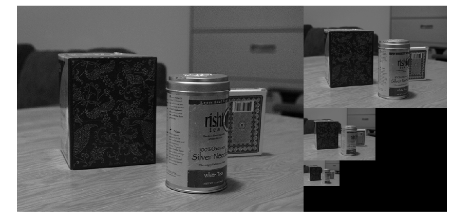
Following is the description of pyramidal Lucas-Kanade algorithm:
Let be a point on image and be the scale of pyramid representation.
- Build pyramid representations of and : and
- Initialize pyramidal guess $$g{L_m}=[g{L_m}_xg{L_m}_y]T=[0\space 0]^T$$
- for to with step of
- Compute location of on :
- Let be the optical flow vector at level :$$dL:=IterativeLucasKanade(IL,JL,pL,g^L)$$
- Guess for next level L−1:
- Return
Implement pyramid_lucas_kanade.
上面的是金字塔法Lukas-Kanade光流的算法描述
1 | from motion import pyramid_lucas_kanade |
2 | |
3 | # Lucas-Kanade method for optical flow |
4 | flow_vectors = pyramid_lucas_kanade(frames[0], frames[1], keypoints) |
5 | |
6 | # Plot flow vectors |
7 | plt.figure(figsize=(15,12)) |
8 | plt.imshow(frames[0]) |
9 | plt.axis('off') |
10 | plt.title('Optical flow vectors (pyramid LK)') |
11 | |
12 | for y, x, vy, vx in np.hstack((keypoints, flow_vectors)): |
13 | plt.arrow(x, y, vx, vy, head_width=3, head_length=3, color='b') |

上图可知,金字塔方式LK光流既能检测到大运行,也能检测到小运动。但是幅度也太大了点。
1 | # Plot tracked kepoints |
2 | new_keypoints = keypoints + flow_vectors |
3 | plt.figure(figsize=(15,12)) |
4 | plt.imshow(frames[1]) |
5 | plt.scatter(new_keypoints[:,1], new_keypoints[:,0], |
6 | facecolors='none', edgecolors='r') |
7 | plt.axis('off') |
8 | plt.title('Tracked keypoints in the second frame (pyramid LK)') |
9 | |
10 | plt.show() |

1 | from utils import animated_scatter |
2 | from motion import track_features |
3 | keypoints = corner_peaks(corner_harris(frames[0]), |
4 | exclude_border=5, |
5 | threshold_rel=0.01) |
6 | |
7 | trajs = track_features(frames, keypoints, |
8 | error_thresh=1.5, |
9 | optflow_fn=pyramid_lucas_kanade, |
10 | window_size=5) |
11 | ani = animated_scatter(frames,trajs) |
12 | HTML(ani.to_html5_video()) |
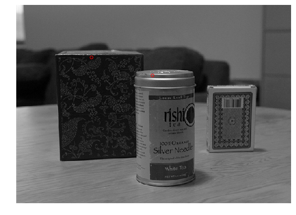
总体比较下来,金字塔法光流耗时最多。
效果也不稳定,貌似第二帧关键点都追丢了,怀疑是计算得到的光流幅度太大引起的。
Object Tracking
Let us build a simple object tracker using the Lucas-Kanade method we have implemented in previous sections. In order to test the object tracker, we provide you a short face-tracking sequence. Each frame in the sequence is annotated with the ground-truth location (as bounding box) of face.
An object tracker is given an object bounding box in the first frame, and it has to track the object by predicting bounding boxes in subsequent frames.
目标追踪
在第一帧中提供了目标的外包围框,要在接下来的帧序列中预测目标运行。
1 | from utils import animated_bbox, load_bboxes |
2 | |
3 | # Load frames and ground truth bounding boxes |
4 | frames = load_frames('Man/img') |
5 | gt_bboxes = load_bboxes('Man/groundtruth_rect.txt') |
6 | |
7 | ani = animated_bbox(frames, gt_bboxes) |
8 | HTML(ani.to_html5_video()) |
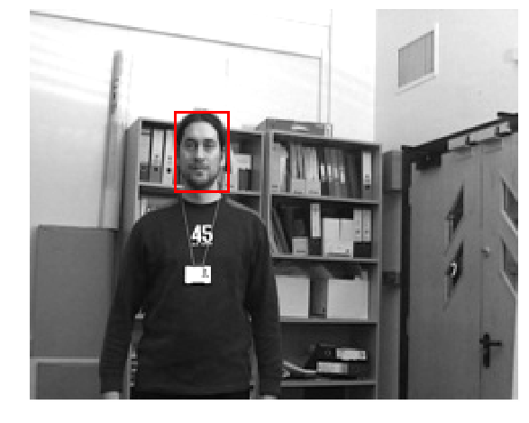
In order to track the object, we first find keypoints to track inside the bounding box. Then, we track those points in each of the following frames and output a tight bounding box around the tracked points. In order to prevent all the keypoints being lost, we detect new keypoints within the bounding box every 20 frames.
找到包围盒中的关键点。
在接下来的帧中追踪这些关键点,并用包围盒框住这些关键点。
为了防止关键点的消失,每二十帧进行一次关键点的检测。
1 | # Find features to track within the bounding box |
2 | x, y, w, h = gt_bboxes[0] |
3 | roi = frames[0][y:y+h, x:x+w] |
4 | keypoints = corner_peaks(corner_harris(roi), |
5 | exclude_border=3, |
6 | threshold_rel=0.001) |
7 | |
8 | # Shift keypoints by bbox offset |
9 | keypoints[:,1] += x |
10 | keypoints[:,0] += y |
11 | |
12 | # Plot kepoints |
13 | plt.figure(figsize=(15,12)) |
14 | plt.imshow(frames[0]) |
15 | plt.scatter(keypoints[:,1], keypoints[:,0], |
16 | facecolors='none', edgecolors='r') |
17 | plt.axis('off') |
18 | plt.show() |
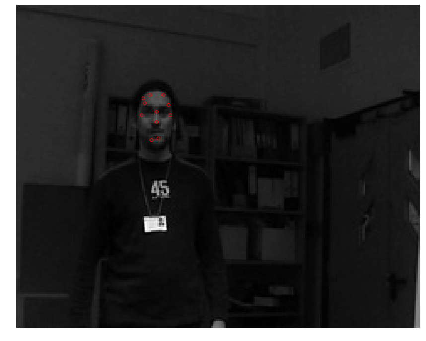
1 | from motion import compute_error |
2 | |
3 | # Initailze keypoints abd bounding box |
4 | kp_I = keypoints |
5 | x, y, w, h = gt_bboxes[0] |
6 | bboxes = [(x, y, w, h)] |
7 | |
8 | for i in range(len(frames)-1): |
9 | I = frames[i] # current frame |
10 | J = frames[i+1] # next frame |
11 | |
12 | # estimate keypoints in frame J |
13 | # 这里使用迭代式LK光流和金字塔LK光流进行测试 |
14 | flow_vectors = iterative_lucas_kanade(I, J, kp_I) #pyramid_lucas_kanade |
15 | kp_J = kp_I + flow_vectors |
16 | |
17 | # Leave out lost points |
18 | new_keypoints = [] |
19 | for yi, xi, yj, xj in np.hstack((kp_I, kp_J)): |
20 | if yj > J.shape[0]-2 or yj < 1 or xj > J.shape[1]-2 or xj < 1: |
21 | print('out of bound') |
22 | continue |
23 | else: |
24 | patch_I = I[int(yi)-1:int(yi)+2, int(xi)-1:int(xi)+2] |
25 | patch_J = J[int(yj)-1:int(yj)+2, int(xj)-1:int(xj)+2] |
26 | error = compute_error(patch_I, patch_J) |
27 | if error > 3.0: |
28 | continue |
29 | else: |
30 | new_keypoints.append([yj, xj]) |
31 | |
32 | # Update keypoints |
33 | kp_I = np.array(new_keypoints) |
34 | |
35 | # Find bounding box around the keypoints |
36 | if len(kp_I) > 0: |
37 | x = int(kp_I[:,1].min()) |
38 | y = int(kp_I[:,0].min()) |
39 | w = int(kp_I[:,1].max()) - x |
40 | h = int(kp_I[:,0].max()) - y |
41 | else: |
42 | (x, y, w, h) = (0, 0, 0, 0) |
43 | bboxes.append((x,y,w,h)) |
44 | |
45 | # Refresh keypoints every 20 frames |
46 | if (i+1) % 20 == 0 and (w * h > 0): |
47 | roi = J[y:y+h, x:x+w] |
48 | new_keypoints = corner_peaks(corner_harris(roi), |
49 | exclude_border=5, |
50 | threshold_rel=0.01) |
51 | new_keypoints[:,1] += x |
52 | new_keypoints[:,0] += y |
53 | kp_I = np.vstack((kp_I, new_keypoints)) |
1 | ani = animated_bbox(frames, bboxes) |
2 | HTML(ani.to_html5_video()) |
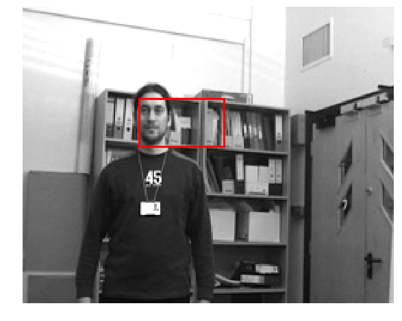
金字塔光流法
到最后竟然包围盒消失了,两个原因吧
- 一个是特征点的检测算法对于光照敏感,
- 一个是光流追踪没有完善。
其实,上一步金字塔光流法其实还没有解决问题哩。
迭代光流法
IOU分数能达到0.32,但是明显的错误在于,在过程中更新关键点时,将复杂背景下的一些脸部之外的关键点包括了进来,导致了最后的追踪不仅包含了最开始的目标,还包括了复杂背景的一些关键点。
Evaluating Object Tracker: intersection over union (IoU)
Intersection over union is a common metric for evaluating performance of an object tracker. Implement IoU in motion.py to evaluate our object tracker. With default parameters, you will get IoU score of ~0.32.
根据真值,评估自己的追踪效果。
计算方法看图:
1 | from motion import IoU |
2 | |
3 | average_iou = 0.0 |
4 | for gt_bbox, bbox in zip(gt_bboxes, bboxes): |
5 | average_iou += IoU(gt_bbox, bbox) |
6 | |
7 | average_iou /= len(gt_bboxes) |
8 | print(average_iou) |
1 | 0.32643400622199703 |
Extra Credit: Optimizing Object Tracker
Optimize object tracker in the code cell below. You may modify the code and define new parameters. We will grant extra credit for IoU score > 0.45.
这里要求改进,提高准确率。
思路就是,从上一视频的问题入手,错误的一个明显原因就是引入了复杂背景的一些关键点,所以一个解决方案就是避免引入这些关键点。
方案一:
- 每隔20帧重新获取关键点
- 对新的关键点进行筛选,保留与初始关键点最相似的点。其实就是根据找特征点的匹配。
这就需要对关键点进行描述了。当然,其实也可以对Harris检测角点这一方法换成别的关键点检测算法来做。