深度学习框架pytorch
前言
所有代码都在当前版本pytorch下测试通过
1 | import torch |
2 | print(torch.__version__) |
3 | print(torch.device('cuda' if torch.cuda.is_available() else 'cpu')) |
1 | 1.1.0.post2 |
2 | cpu |
pytorch基础
autograd 求取梯度
- 导入包
1 | import torch |
2 | import torchvision |
3 | import torch.nn as nn |
4 | import numpy as np |
5 | import torchvision.transforms as transforms |
- autograd(自动求导/求梯度)
1 | # 创建张量(tensors) |
2 | x = torch.tensor(1., requires_grad=True) |
3 | w = torch.tensor(2., requires_grad=True) |
4 | b = torch.tensor(3., requires_grad=True) |
5 | |
6 | # 构建计算图( computational graph):前向计算 |
7 | y = w * x + b # y = 2 * x + 3 |
8 | |
9 | # 反向传播,计算梯度(gradients) |
10 | y.backward() |
11 | |
12 | # 输出梯度 |
13 | print(x.grad) # x.grad = 2 |
14 | print(w.grad) # w.grad = 1 |
15 | print(b.grad) # b.grad = 1 |
1 | tensor(2.) |
2 | tensor(1.) |
3 | tensor(1.) |
- autograd(自动求导/求梯度)
1 | # 创建大小为 (10, 3) 和 (10, 2)的张量. |
2 | # randn 返回标准正态分布(均值为0,方差为1)的随机数, rand返回区间(0,1)均匀分布的随机数 |
3 | x = torch.randn(10, 3) |
4 | y = torch.randn(10, 2) |
5 | |
6 | # 构建全连接层(fully connected layer) |
7 | linear = nn.Linear(3, 2) |
8 | print ('w: ', linear.weight) |
9 | print ('b: ', linear.bias) |
10 | |
11 | # 构建损失函数和优化器(loss function and optimizer) |
12 | # 损失函数使用均方差 |
13 | # 优化器使用随机梯度下降,lr是learning rate |
14 | criterion = nn.MSELoss() |
15 | optimizer = torch.optim.SGD(linear.parameters(), lr=0.01) |
16 | |
17 | # 前向传播 |
18 | pred = linear(x) |
19 | |
20 | # 计算损失 |
21 | loss = criterion(pred, y) |
22 | print('loss: ', loss.item()) |
23 | |
24 | # 反向传播 |
25 | loss.backward() |
26 | |
27 | # 输出梯度 |
28 | print ('dL/dw: ', linear.weight.grad) |
29 | print ('dL/db: ', linear.bias.grad) |
30 | |
31 | # 执行一步-梯度下降(1-step gradient descent) |
32 | optimizer.step() |
33 | |
34 | # 更底层的实现方式是这样子的 |
35 | # linear.weight.data.sub_(0.01 * linear.weight.grad.data) |
36 | # linear.bias.data.sub_(0.01 * linear.bias.grad.data) |
37 | |
38 | # 进行一次梯度下降之后,输出新的预测损失 |
39 | # loss的确变少了 |
40 | pred = linear(x) |
41 | loss = criterion(pred, y) |
42 | print('loss after 1 step optimization: ', loss.item()) |
1 | w: Parameter containing: |
2 | tensor([[-0.3414, -0.2485, 0.5127], |
3 | [ 0.1081, -0.2054, -0.0197]], requires_grad=True) |
4 | b: Parameter containing: |
5 | tensor([ 0.0694, -0.4127], requires_grad=True) |
6 | loss: 1.1263189315795898 |
7 | dL/dw: tensor([[-0.8668, -0.4168, 0.2444], |
8 | [ 0.5876, -0.0610, 0.4616]]) |
9 | dL/db: tensor([ 0.0916, -0.3413]) |
10 | loss after 1 step optimization: 1.1097254753112793 |
从Numpy装载数据
1 | # 创建Numpy数组 |
2 | x = np.array([[1, 2], [3, 4]]) |
3 | print(x) |
4 | |
5 | # 将numpy数组转换为torch的张量 |
6 | y = torch.from_numpy(x) |
7 | print(y) |
8 | |
9 | # 将torch的张量转换为numpy数组 |
10 | z = y.numpy() |
11 | print(z) |
1 | [[1 2] |
2 | [3 4]] |
3 | tensor([[1, 2], |
4 | [3, 4]]) |
5 | [[1 2] |
6 | [3 4]] |
输入工作流(Input pipeline)
1 | # 下载和构造CIFAR-10 数据集 |
2 | # Cifar-10数据集介绍:https://www.cs.toronto.edu/~kriz/cifar.html |
3 | train_dataset = torchvision.datasets.CIFAR10(root='../../../data/', |
4 | train=True, |
5 | transform=transforms.ToTensor(), |
6 | download=True) |
7 | |
8 | # 获取一组数据对(从磁盘中读取) |
9 | image, label = train_dataset[0] |
10 | print (image.size()) |
11 | print (label) |
12 | |
13 | # 数据加载器(提供了队列和线程的简单实现) |
14 | train_loader = torch.utils.data.DataLoader(dataset=train_dataset, |
15 | batch_size=64, |
16 | shuffle=True) |
17 | |
18 | # 迭代的使用 |
19 | # 当迭代开始时,队列和线程开始从文件中加载数据 |
20 | data_iter = iter(train_loader) |
21 | |
22 | # 获取一组mini-batch |
23 | images, labels = data_iter.next() |
24 | |
25 | |
26 | # 正常的使用方式如下: |
27 | for images, labels in train_loader: |
28 | # 在此处添加训练用的代码 |
29 | pass |
1 | Files already downloaded and verified |
2 | torch.Size([3, 32, 32]) |
3 | 6 |
自定义数据集的Input pipeline
1 | # 构建自定义数据集的方式如下: |
2 | class CustomDataset(torch.utils.data.Dataset): |
3 | def __init__(self): |
4 | # TODO |
5 | # 1. 初始化文件路径或者文件名 |
6 | pass |
7 | def __getitem__(self, index): |
8 | # TODO |
9 | # 1. 从文件中读取一份数据(比如使用nump.fromfile,PIL.Image.open) |
10 | # 2. 预处理数据(比如使用 torchvision.Transform) |
11 | # 3. 返回数据对(比如 image和label) |
12 | pass |
13 | def __len__(self): |
14 | # 将0替换成数据集的总长度 |
15 | return 0 |
16 | |
17 | # 然后就可以使用预置的数据加载器(data loader)了 |
18 | custom_dataset = CustomDataset() |
19 | train_loader = torch.utils.data.DataLoader(dataset=custom_dataset, |
20 | batch_size=64, |
21 | shuffle=True) |
如果没有实现TODO会报错误
1 | --------------------------------------------------------------------------- |
2 | ValueError Traceback (most recent call last) |
3 | <ipython-input-27-be02a903d589> in <module> |
4 | 1 train_loader = torch.utils.data.DataLoader(dataset=custom_dataset, |
5 | 2 batch_size=64, |
6 | ----> 3 shuffle=True) |
7 | |
8 | /usr/local/Cellar/python/3.7.3/Frameworks/Python.framework/Versions/3.7/lib/python3.7/site-packages/torch/utils/data/dataloader.py in __init__(self, dataset, batch_size, shuffle, sampler, batch_sampler, num_workers, collate_fn, pin_memory, drop_last, timeout, worker_init_fn) |
9 | 174 if sampler is None: |
10 | 175 if shuffle: |
11 | --> 176 sampler = RandomSampler(dataset) |
12 | 177 else: |
13 | 178 sampler = SequentialSampler(dataset) |
14 | |
15 | /usr/local/Cellar/python/3.7.3/Frameworks/Python.framework/Versions/3.7/lib/python3.7/site-packages/torch/utils/data/sampler.py in __init__(self, data_source, replacement, num_samples) |
16 | 64 if not isinstance(self.num_samples, int) or self.num_samples <= 0: |
17 | 65 raise ValueError("num_samples should be a positive integer " |
18 | ---> 66 "value, but got num_samples={}".format(self.num_samples)) |
19 | 67 |
20 | 68 @property |
21 | |
22 | ValueError: num_samples should be a positive integer value, but got num_samples=0 |
预训练模型
1 | # 下载并加载预训练好的模型 ResNet-18 |
2 | resnet = torchvision.models.resnet18(pretrained=True) |
3 | |
4 | # 如果想要在模型仅对Top Layer进行微调的话,可以设置如下: |
5 | # requieres_grad设置为False的话,就不会进行梯度更新,就能保持原有的参数 |
6 | for param in resnet.parameters(): |
7 | param.requires_grad = False |
8 | |
9 | # 替换TopLayer,只对这一层做微调 |
10 | resnet.fc = nn.Linear(resnet.fc.in_features, 100) # 100 is an example. |
11 | |
12 | # 前向传播 |
13 | images = torch.randn(64, 3, 224, 224) |
14 | outputs = resnet(images) |
15 | print (outputs.size()) # (64, 100) |
1 | torch.Size([64, 100]) |
保存和加载模型
1 | # 保存和加载整个模型 |
2 | torch.save(resnet, 'model.ckpt') |
3 | model = torch.load('model.ckpt') |
4 | |
5 | # 仅保存和加载模型的参数(推荐这个方式) |
6 | torch.save(resnet.state_dict(), 'params.ckpt') |
7 | resnet.load_state_dict(torch.load('params.ckpt')) |
线性回归(Linear Regression)
- 导入包
1 | import torch |
2 | import torch.nn as nn |
3 | import numpy as np |
4 | import matplotlib.pyplot as plt |
- 参数、模型设置
1 | # 超参数设置 |
2 | input_size = 1 |
3 | output_size = 1 |
4 | num_epochs = 60 |
5 | learning_rate = 0.001 |
6 | |
7 | # Toy dataset |
8 | # 玩具资料:小数据集 |
9 | x_train = np.array([[3.3], [4.4], [5.5], [6.71], [6.93], [4.168], |
10 | [9.779], [6.182], [7.59], [2.167], [7.042], |
11 | [10.791], [5.313], [7.997], [3.1]], dtype=np.float32) |
12 | |
13 | y_train = np.array([[1.7], [2.76], [2.09], [3.19], [1.694], [1.573], |
14 | [3.366], [2.596], [2.53], [1.221], [2.827], |
15 | [3.465], [1.65], [2.904], [1.3]], dtype=np.float32) |
16 | |
17 | # 线性回归模型 |
18 | model = nn.Linear(input_size, output_size) |
19 | |
20 | # 损失函数和优化器 |
21 | criterion = nn.MSELoss() |
22 | optimizer = torch.optim.SGD(model.parameters(), lr=learning_rate) |
- 训练模型
1 | for epoch in range(num_epochs): |
2 | # 将Numpy数组转换为torch张量 |
3 | inputs = torch.from_numpy(x_train) |
4 | targets = torch.from_numpy(y_train) |
5 | |
6 | # 前向传播 |
7 | outputs = model(inputs) |
8 | loss = criterion(outputs, targets) |
9 | |
10 | # 反向传播和优化 |
11 | optimizer.zero_grad() |
12 | loss.backward() |
13 | optimizer.step() |
14 | |
15 | if (epoch+1) % 5 == 0: |
16 | print ('Epoch [{}/{}], Loss: {:.4f}'.format(epoch+1, num_epochs, loss.item())) |
1 | Epoch [5/60], Loss: 7.4997 |
2 | Epoch [10/60], Loss: 3.1402 |
3 | Epoch [15/60], Loss: 1.3741 |
4 | Epoch [20/60], Loss: 0.6586 |
5 | Epoch [25/60], Loss: 0.3687 |
6 | Epoch [30/60], Loss: 0.2513 |
7 | Epoch [35/60], Loss: 0.2037 |
8 | Epoch [40/60], Loss: 0.1844 |
9 | Epoch [45/60], Loss: 0.1766 |
10 | Epoch [50/60], Loss: 0.1734 |
11 | Epoch [55/60], Loss: 0.1722 |
12 | Epoch [60/60], Loss: 0.1716 |
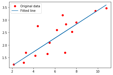
- 绘制图形
1 | # torch.from_numpy(x_train)将X_train转换为Tensor |
2 | # model()根据输入和模型,得到输出 |
3 | # detach().numpy()预测结结果转换为numpy数组 |
4 | predicted = model(torch.from_numpy(x_train)).detach().numpy() |
5 | plt.plot(x_train, y_train, 'ro', label='Original data') |
6 | plt.plot(x_train, predicted, label='Fitted line') |
7 | plt.legend() |
8 | plt.show() |
- 将模型的记录节点保存下来
1 | torch.save(model.state_dict(), 'model.ckpt') |
逻辑回归(Logistic Regression)
- 导入包
1 | import torch |
2 | import torch.nn as nn |
3 | import torchvision |
4 | import torchvision.transforms as transforms |
- 参数设置
1 | # 超参数设置 Hyper-parameters |
2 | input_size = 784 |
3 | num_classes = 10 |
4 | num_epochs = 5 |
5 | batch_size = 100 |
6 | learning_rate = 0.001 |
- MINIST数据集加载(image and labels)
1 | train_dataset = torchvision.datasets.MNIST(root='../../../data/minist', |
2 | train=True, |
3 | transform=transforms.ToTensor(), |
4 | download=True) |
1 | Downloading http://yann.lecun.com/exdb/mnist/train-images-idx3-ubyte.gz to ../../../data/minist/MNIST/raw/train-images-idx3-ubyte.gz |
2 | 100.1% |
3 | Extracting ../../../data/minist/MNIST/raw/train-images-idx3-ubyte.gz |
4 | Downloading http://yann.lecun.com/exdb/mnist/train-labels-idx1-ubyte.gz to ../../../data/minist/MNIST/raw/train-labels-idx1-ubyte.gz |
5 | 113.5% |
6 | Extracting ../../../data/minist/MNIST/raw/train-labels-idx1-ubyte.gz |
7 | Downloading http://yann.lecun.com/exdb/mnist/t10k-images-idx3-ubyte.gz to ../../../data/minist/MNIST/raw/t10k-images-idx3-ubyte.gz |
8 | 100.4% |
9 | Extracting ../../../data/minist/MNIST/raw/t10k-images-idx3-ubyte.gz |
10 | Downloading http://yann.lecun.com/exdb/mnist/t10k-labels-idx1-ubyte.gz to ../../../data/minist/MNIST/raw/t10k-labels-idx1-ubyte.gz |
11 | 180.4% |
12 | Extracting ../../../data/minist/MNIST/raw/t10k-labels-idx1-ubyte.gz |
13 | Processing... |
14 | Done! |
1 | test_dataset = torchvision.datasets.MNIST(root='../../../data/minist', |
2 | train=False, |
3 | transform=transforms.ToTensor()) |
1 | # 数据加载器(data loader) |
2 | train_loader = torch.utils.data.DataLoader(dataset=train_dataset, |
3 | batch_size=batch_size, |
4 | shuffle=True) |
5 | |
6 | test_loader = torch.utils.data.DataLoader(dataset=test_dataset, |
7 | batch_size=batch_size, |
8 | shuffle=False) |
- Logistic Regression模型:加载和训练
1 | # 线性模型,指定 |
2 | model = nn.Linear(input_size, num_classes) |
3 | |
4 | # 损失函数和优化器 |
5 | # nn.CrossEntropyLoss()内部集成了softmax函数 |
6 | # It is useful when training a classification problem with `C` classes. |
7 | criterion = nn.CrossEntropyLoss() |
8 | optimizer = torch.optim.SGD(model.parameters(), lr=learning_rate) |
9 | |
10 | # 训练模型 |
11 | total_step = len(train_loader) |
12 | for epoch in range(num_epochs): |
13 | for i, (images, labels) in enumerate(train_loader): |
14 | # 将图像序列抓换至大小为 (batch_size, input_size) |
15 | images = images.reshape(-1, 28*28) |
16 | |
17 | # 前向传播 |
18 | outputs = model(images) |
19 | loss = criterion(outputs, labels) |
20 | |
21 | # 反向传播及优化 |
22 | optimizer.zero_grad() # 注意每次循环都要注意清空梯度缓存 |
23 | loss.backward() |
24 | optimizer.step() |
25 | |
26 | if (i+1) % 100 == 0: |
27 | print ('Epoch [{}/{}], Step [{}/{}], Loss: {:.4f}' |
28 | .format(epoch+1, num_epochs, i+1, total_step, loss.item())) |
1 | Epoch [1/5], Step [100/600], Loss: 2.2573 |
2 | Epoch [1/5], Step [200/600], Loss: 2.1257 |
3 | Epoch [1/5], Step [300/600], Loss: 2.0524 |
4 | Epoch [1/5], Step [400/600], Loss: 1.9810 |
5 | Epoch [1/5], Step [500/600], Loss: 1.9118 |
6 | Epoch [1/5], Step [600/600], Loss: 1.8635 |
7 | Epoch [2/5], Step [100/600], Loss: 1.7000 |
8 | Epoch [2/5], Step [200/600], Loss: 1.7233 |
9 | Epoch [2/5], Step [300/600], Loss: 1.6955 |
10 | Epoch [2/5], Step [400/600], Loss: 1.5738 |
11 | Epoch [2/5], Step [500/600], Loss: 1.6119 |
12 | Epoch [2/5], Step [600/600], Loss: 1.4994 |
13 | Epoch [3/5], Step [100/600], Loss: 1.4966 |
14 | Epoch [3/5], Step [200/600], Loss: 1.3909 |
15 | Epoch [3/5], Step [300/600], Loss: 1.2951 |
16 | Epoch [3/5], Step [400/600], Loss: 1.3250 |
17 | Epoch [3/5], Step [500/600], Loss: 1.1628 |
18 | Epoch [3/5], Step [600/600], Loss: 1.2553 |
19 | Epoch [4/5], Step [100/600], Loss: 1.2861 |
20 | Epoch [4/5], Step [200/600], Loss: 1.1990 |
21 | Epoch [4/5], Step [300/600], Loss: 1.2871 |
22 | Epoch [4/5], Step [400/600], Loss: 1.1154 |
23 | Epoch [4/5], Step [500/600], Loss: 1.1758 |
24 | Epoch [4/5], Step [600/600], Loss: 1.1805 |
25 | Epoch [5/5], Step [100/600], Loss: 1.0249 |
26 | Epoch [5/5], Step [200/600], Loss: 1.0673 |
27 | Epoch [5/5], Step [300/600], Loss: 1.0265 |
28 | Epoch [5/5], Step [400/600], Loss: 1.0038 |
29 | Epoch [5/5], Step [500/600], Loss: 1.0607 |
30 | Epoch [5/5], Step [600/600], Loss: 1.0184 |
- 模型测试
1 | # 在测试阶段,为了运行内存效率,就不需要计算梯度了 |
2 | # PyTorch 默认每一次前向传播都会计算梯度 |
3 | with torch.no_grad(): |
4 | correct = 0 |
5 | total = 0 |
6 | for images, labels in test_loader: |
7 | images = images.reshape(-1, 28*28) |
8 | outputs = model(images) |
9 | _, predicted = torch.max(outputs.data, 1) |
10 | total += labels.size(0) |
11 | correct += (predicted == labels).sum() |
12 | |
13 | print('Accuracy of the model on the 10000 test images: {} %'.format(100 * correct / total)) |
1 | Accuracy of the model on the 10000 test images: 82 % |
- 保存模型
1 | torch.save(model.state_dict(), 'model.ckpt') |
前馈神经网络(Feedforward Neural Network)
- 导入包
1 | import torch |
2 | import torch.nn as nn |
3 | import torchvision |
4 | import torchvision.transforms as transforms |
- 参数设置
1 | # 设备配置 |
2 | # 有cuda就用cuda |
3 | device = torch.device('cuda' if torch.cuda.is_available() else 'cpu') |
4 | |
5 | # 超参数设置 |
6 | input_size = 784 |
7 | hidden_size = 500 |
8 | num_classes = 10 |
9 | num_epochs = 5 |
10 | batch_size = 100 |
11 | learning_rate = 0.001 |
- MINIST 数据集加载
1 | # 训练数据集 |
2 | train_dataset = torchvision.datasets.MNIST(root='../../../data/minist', |
3 | train=True, |
4 | transform=transforms.ToTensor(), |
5 | download=True) |
1 | # 测试数据集 |
2 | test_dataset = torchvision.datasets.MNIST(root='../../../data/minist', |
3 | train=False, |
4 | transform=transforms.ToTensor()) |
1 | # 数据加载器 Data Loader |
2 | # 训练数据加载器 |
3 | train_loader = torch.utils.data.DataLoader(dataset=train_dataset, |
4 | batch_size=batch_size, |
5 | shuffle=True) |
6 | |
7 | # 测试数据加载器 |
8 | test_loader = torch.utils.data.DataLoader(dataset=test_dataset, |
9 | batch_size=batch_size, |
10 | shuffle=False) |
- 自定义前馈神经网络
1 | # 定义:有一个隐藏层的全连接的神经网络 |
2 | class NeuralNet(nn.Module): |
3 | def __init__(self, input_size, hidden_size, num_classes): |
4 | super(NeuralNet, self).__init__() |
5 | self.fc1 = nn.Linear(input_size, hidden_size) |
6 | self.relu = nn.ReLU() |
7 | self.fc2 = nn.Linear(hidden_size, num_classes) |
8 | |
9 | def forward(self, x): |
10 | out = self.fc1(x) |
11 | out = self.relu(out) |
12 | out = self.fc2(out) |
13 | return out |
1 | # 加载(实例化)一个网络模型 |
2 | # to(device)可以用来将模型放在GPU上训练 |
3 | model = NeuralNet(input_size, hidden_size, num_classes).to(device) |
4 | |
5 | # 定义损失函数和优化器 |
6 | # 再次,损失函数CrossEntropyLoss适合用于分类问题,因为它自带SoftMax功能 |
7 | criterion = nn.CrossEntropyLoss() |
8 | optimizer = torch.optim.Adam(model.parameters(), lr=learning_rate) |
- 训练模型
1 | total_step = len(train_loader) |
2 | |
3 | for epoch in range(num_epochs): |
4 | for i, (images, labels) in enumerate(train_loader): |
5 | # 将tensor移动到配置好的设备上(GPU) |
6 | images = images.reshape(-1, 28*28).to(device) |
7 | labels = labels.to(device) |
8 | |
9 | # 前向传播 |
10 | outputs = model(images) |
11 | loss = criterion(outputs, labels) |
12 | |
13 | # 反向传播和优化 |
14 | optimizer.zero_grad() # 还是要注意此处,每次迭代训练都需要清空梯度缓存 |
15 | loss.backward() |
16 | optimizer.step() |
17 | |
18 | if (i+1) % 100 == 0: |
19 | print ('Epoch [{}/{}], Step [{}/{}], Loss: {:.4f}' |
20 | .format(epoch+1, num_epochs, i+1, total_step, loss.item())) |
1 | Epoch [1/5], Step [100/600], Loss: 0.3046 |
2 | Epoch [1/5], Step [200/600], Loss: 0.2803 |
3 | Epoch [1/5], Step [300/600], Loss: 0.2142 |
4 | Epoch [1/5], Step [400/600], Loss: 0.1459 |
5 | Epoch [1/5], Step [500/600], Loss: 0.1378 |
6 | Epoch [1/5], Step [600/600], Loss: 0.2241 |
7 | Epoch [2/5], Step [100/600], Loss: 0.1013 |
8 | Epoch [2/5], Step [200/600], Loss: 0.0935 |
9 | Epoch [2/5], Step [300/600], Loss: 0.0990 |
10 | Epoch [2/5], Step [400/600], Loss: 0.1639 |
11 | Epoch [2/5], Step [500/600], Loss: 0.0283 |
12 | Epoch [2/5], Step [600/600], Loss: 0.0304 |
13 | Epoch [3/5], Step [100/600], Loss: 0.0659 |
14 | Epoch [3/5], Step [200/600], Loss: 0.0738 |
15 | Epoch [3/5], Step [300/600], Loss: 0.1491 |
16 | Epoch [3/5], Step [400/600], Loss: 0.1034 |
17 | Epoch [3/5], Step [500/600], Loss: 0.0109 |
18 | Epoch [3/5], Step [600/600], Loss: 0.0884 |
19 | Epoch [4/5], Step [100/600], Loss: 0.0489 |
20 | Epoch [4/5], Step [200/600], Loss: 0.0575 |
21 | Epoch [4/5], Step [300/600], Loss: 0.0833 |
22 | Epoch [4/5], Step [400/600], Loss: 0.0684 |
23 | Epoch [4/5], Step [500/600], Loss: 0.0445 |
24 | Epoch [4/5], Step [600/600], Loss: 0.0789 |
25 | Epoch [5/5], Step [100/600], Loss: 0.0192 |
26 | Epoch [5/5], Step [200/600], Loss: 0.0227 |
27 | Epoch [5/5], Step [300/600], Loss: 0.0076 |
28 | Epoch [5/5], Step [400/600], Loss: 0.0595 |
29 | Epoch [5/5], Step [500/600], Loss: 0.0214 |
30 | Epoch [5/5], Step [600/600], Loss: 0.0562 |
- 测试并保存模型
1 | # 测试阶段为提高效率,可以不计算梯度 |
2 | # 使用with torch.no_grad()函数 |
3 | |
4 | with torch.no_grad(): |
5 | correct = 0 |
6 | total = 0 |
7 | for images, labels in test_loader: |
8 | images = images.reshape(-1, 28*28).to(device) |
9 | labels = labels.to(device) |
10 | outputs = model(images) |
11 | # 统计预测概率最大的下标 |
12 | _, predicted = torch.max(outputs.data, 1) |
13 | total += labels.size(0) |
14 | correct += (predicted == labels).sum().item() |
15 | |
16 | print('Accuracy of the network on the 10000 test images: {} %'.format(100 * correct / total)) |
1 | Accuracy of the network on the 10000 test images: 97.73 % |
- 保存模型
1 | torch.save(model.state_dict(), 'model.ckpt') |
卷积神经网络(Convolutional Neural Network)
- 导入包
1 | import torch |
2 | import torch.nn as nn |
3 | import torchvision |
4 | import torchvision.transforms as transforms |
- 参数设置
1 | # 设备配置 |
2 | device = torch.device('cuda' if torch.cuda.is_available() else 'cpu') |
3 | if device.type != 'cpu': |
4 | torch.cuda.set_device(1) # 这句用来设置pytorch在哪块GPU上运行 |
5 | |
6 | # 超参数设置 |
7 | num_epochs = 5 |
8 | num_classes = 10 |
9 | batch_size = 100 |
10 | learning_rate = 0.001 |
- MINIST数据集
1 | # 训练数据集 |
2 | train_dataset = torchvision.datasets.MNIST(root='../../../data/minist/', |
3 | train=True, |
4 | transform=transforms.ToTensor(), |
5 | download=True) |
6 | |
7 | # 测试数据集 |
8 | test_dataset = torchvision.datasets.MNIST(root='../../../data/minist', |
9 | train=False, |
10 | transform=transforms.ToTensor()) |
11 | |
12 | # 数据加载器 |
13 | # 训练数据 加载器 |
14 | train_loader = torch.utils.data.DataLoader(dataset=train_dataset, |
15 | batch_size=batch_size, |
16 | shuffle=True) |
17 | |
18 | # 测试数据加载器 |
19 | test_loader = torch.utils.data.DataLoader(dataset=test_dataset, |
20 | batch_size=batch_size, |
21 | shuffle=False) |
- 自定义 卷积神经网络
1 | # 搭建卷积神经网络模型 |
2 | # 两个卷积层 |
3 | class ConvNet(nn.Module): |
4 | def __init__(self, num_classes=10): |
5 | super(ConvNet, self).__init__() |
6 | self.layer1 = nn.Sequential( |
7 | # 卷积层计算 |
8 | nn.Conv2d(1, 16, kernel_size=5, stride=1, padding=2), |
9 | # 批归一化 |
10 | nn.BatchNorm2d(16), |
11 | #ReLU激活函数 |
12 | nn.ReLU(), |
13 | # 池化层:最大池化 |
14 | nn.MaxPool2d(kernel_size=2, stride=2)) |
15 | self.layer2 = nn.Sequential( |
16 | nn.Conv2d(16, 32, kernel_size=5, stride=1, padding=2), |
17 | nn.BatchNorm2d(32), |
18 | nn.ReLU(), |
19 | nn.MaxPool2d(kernel_size=2, stride=2)) |
20 | self.fc = nn.Linear(7*7*32, num_classes) |
21 | |
22 | # 定义前向传播顺序 |
23 | def forward(self, x): |
24 | out = self.layer1(x) |
25 | out = self.layer2(out) |
26 | out = out.reshape(out.size(0), -1) |
27 | out = self.fc(out) |
28 | return out |
1 | # 实例化一个模型,并迁移至gpu|cpu |
2 | model = ConvNet(num_classes).to(device) |
3 | |
4 | # 定义损失函数和优化器 |
5 | criterion = nn.CrossEntropyLoss() |
6 | optimizer = torch.optim.Adam(model.parameters(), lr=learning_rate) |
- 训练模型
1 | total_step = len(train_loader) |
2 | for epoch in range(num_epochs): |
3 | for i, (images, labels) in enumerate(train_loader): |
4 | # 注意模型在GPU中,数据也要搬到GPU中 |
5 | images = images.to(device) |
6 | labels = labels.to(device) |
7 | |
8 | # 前向传播 |
9 | outputs = model(images) |
10 | loss = criterion(outputs, labels) |
11 | |
12 | # 反向传播和优化 |
13 | optimizer.zero_grad() |
14 | loss.backward() |
15 | optimizer.step() |
16 | |
17 | if (i+1) % 100 == 0: |
18 | print ('Epoch [{}/{}], Step [{}/{}], Loss: {:.4f}' |
19 | .format(epoch+1, num_epochs, i+1, total_step, loss.item())) |
1 | Epoch [1/5], Step [100/600], Loss: 0.1633 |
2 | Epoch [1/5], Step [200/600], Loss: 0.1629 |
3 | Epoch [1/5], Step [300/600], Loss: 0.0813 |
4 | Epoch [1/5], Step [400/600], Loss: 0.0428 |
5 | Epoch [1/5], Step [500/600], Loss: 0.0351 |
6 | Epoch [1/5], Step [600/600], Loss: 0.1182 |
7 | Epoch [2/5], Step [100/600], Loss: 0.0323 |
8 | Epoch [2/5], Step [200/600], Loss: 0.0501 |
9 | Epoch [2/5], Step [300/600], Loss: 0.0592 |
10 | Epoch [2/5], Step [400/600], Loss: 0.0257 |
11 | Epoch [2/5], Step [500/600], Loss: 0.0668 |
12 | Epoch [2/5], Step [600/600], Loss: 0.0521 |
13 | Epoch [3/5], Step [100/600], Loss: 0.0144 |
14 | Epoch [3/5], Step [200/600], Loss: 0.0292 |
15 | Epoch [3/5], Step [300/600], Loss: 0.0239 |
16 | Epoch [3/5], Step [400/600], Loss: 0.0948 |
17 | Epoch [3/5], Step [500/600], Loss: 0.0140 |
18 | Epoch [3/5], Step [600/600], Loss: 0.0481 |
19 | Epoch [4/5], Step [100/600], Loss: 0.0648 |
20 | Epoch [4/5], Step [200/600], Loss: 0.0362 |
21 | Epoch [4/5], Step [300/600], Loss: 0.0217 |
22 | Epoch [4/5], Step [400/600], Loss: 0.0257 |
23 | Epoch [4/5], Step [500/600], Loss: 0.0833 |
24 | Epoch [4/5], Step [600/600], Loss: 0.0321 |
25 | Epoch [5/5], Step [100/600], Loss: 0.0119 |
26 | Epoch [5/5], Step [200/600], Loss: 0.0307 |
27 | Epoch [5/5], Step [300/600], Loss: 0.0212 |
28 | Epoch [5/5], Step [400/600], Loss: 0.0084 |
29 | Epoch [5/5], Step [500/600], Loss: 0.0159 |
30 | Epoch [5/5], Step [600/600], Loss: 0.0050 |
- 测试并保存模型
1 | # 切换成评估测试模式 |
2 | # 这是因为在测试时,与训练时的dropout和batch normalization的操作是不同的 |
3 | model.eval() |
1 | ConvNet( |
2 | (layer1): Sequential( |
3 | (0): Conv2d(1, 16, kernel_size=(5, 5), stride=(1, 1), padding=(2, 2)) |
4 | (1): BatchNorm2d(16, eps=1e-05, momentum=0.1, affine=True, track_running_stats=True) |
5 | (2): ReLU() |
6 | (3): MaxPool2d(kernel_size=2, stride=2, padding=0, dilation=1, ceil_mode=False) |
7 | ) |
8 | (layer2): Sequential( |
9 | (0): Conv2d(16, 32, kernel_size=(5, 5), stride=(1, 1), padding=(2, 2)) |
10 | (1): BatchNorm2d(32, eps=1e-05, momentum=0.1, affine=True, track_running_stats=True) |
11 | (2): ReLU() |
12 | (3): MaxPool2d(kernel_size=2, stride=2, padding=0, dilation=1, ceil_mode=False) |
13 | ) |
14 | (fc): Linear(in_features=1568, out_features=10, bias=True) |
15 | ) |
1 | # 节省计算资源,不去计算梯度 |
2 | with torch.no_grad(): |
3 | correct = 0 |
4 | total = 0 |
5 | for images, labels in test_loader: |
6 | images = images.to(device) |
7 | labels = labels.to(device) |
8 | outputs = model(images) |
9 | _, predicted = torch.max(outputs.data, 1) |
10 | total += labels.size(0) |
11 | correct += (predicted == labels).sum().item() |
12 | |
13 | print('Test Accuracy of the model on the 10000 test images: {} %'.format(100 * correct / total)) |
1 | Test Accuracy of the model on the 10000 test images: 98.98 % |
- 保存模型
1 | torch.save(model.state_dict(), 'model.ckpt') |
用自己的图片和模型进行测试(单张)
1 | import matplotlib.pyplot as plt # plt 用于显示图片 |
2 | import matplotlib.image as mpimg # mpimg 用于读取图片 |
3 | import numpy as np |
4 | |
5 | #resize功能 |
6 | from PIL import Image |
7 | |
8 | # 彩图转灰度 |
9 | def rgb2gray(rgb): |
10 | return np.dot(rgb[...,:3], [0.299, 0.587, 0.114]) |
11 | |
12 | # 读取图像 |
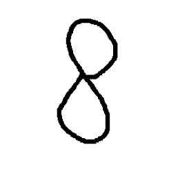
13 | srcPath = '8.png' |
14 | src = mpimg.imread(srcPath)# 读取和代码处于同一目录下的 图片 |
15 | # 此时 lena 就已经是一个 np.array 了,可以对它进行任意处理 |
16 | # 原图大小 |
17 | print(src.shape) |
18 | |
19 | plt.imshow(src) # 显示图片 |
20 | plt.axis('off') # 不显示坐标轴 |
21 | plt.show() |
1 | (252, 261, 4) |
1 | # 转灰度 |
2 | gray = rgb2gray(src) |
3 | |
4 | # 第二个参数如果是整数,则为百分比,如果是tuple,则为输出图像的尺寸 |
5 | gray_new_sz = np.array(Image.fromarray(gray).resize((28,28))) |
6 | print(gray_new_sz.shape) |
7 | plt.imshow(gray_new_sz, cmap='Greys_r') |
8 | plt.axis('off') |
1 | (28, 28) |

1 | # 转换为(B,C,H,W)大小 |
2 | image = gray_new_sz.reshape(-1,1,28,28) |
3 | |
4 | # 转换为torch tensor |
5 | image_tensor = torch.from_numpy(image).float() |
1 | # 调用模型进行评估 |
2 | model.eval() |
3 | |
4 | output = model(image_tensor.to(device)) |
5 | _, predicted = torch.max(output.data, 1) |
6 | pre = predicted.cpu().numpy() |
7 | print(pre) # 查看预测结果 |
1 | 8 |
查看Pytorch跑在哪块GPU上
如果在GPU环境下运行,遇到cuda runtime error: out of memory时,可以查看一下跑在哪块GPU上了。然后用nvidia-smi看一下是不是GPU被占用了。
1 | # 这一段可以用来查看当前GPU的情况 |
2 | import torch |
3 | import sys |
4 | print('__Python VERSION:', sys.version) |
5 | print('__pyTorch VERSION:', torch.__version__) |
6 | print('__CUDA VERSION') |
7 | from subprocess import call |
8 | |
9 | # call(["nvcc", "--version"]) does not work |
10 | ! nvcc --version |
11 | print('__CUDNN VERSION:', torch.backends.cudnn.version()) |
12 | print('__Number CUDA Devices:', torch.cuda.device_count()) |
13 | print('__Devices') |
14 | call(["nvidia-smi", "--format=csv", "--query-gpu=index,name,driver_version,memory.total,memory.used,memory.free"]) |
15 | print('Active CUDA Device: GPU', torch.cuda.current_device()) |
16 | |
17 | print ('Available devices ', torch.cuda.device_count()) |
18 | print ('Current cuda device ', torch.cuda.current_device()) |
深度残差网络(Deep Residual Networks)
根据原文【4.2. CIFAR-10 and Analysis】一节设计的针对数据集CIFAR-10的深度残差网络。
- 预处理
1 | import torch |
2 | import torch.nn as nn |
3 | import torchvision |
4 | import torchvision.transforms as transforms |
1 | # 设备配置 |
2 | torch.cuda.set_device(1) # 这句用来设置pytorch在哪块GPU上运行 |
3 | device = torch.device('cuda' if torch.cuda.is_available() else 'cpu') |
4 | |
5 | # 超参数设置 |
6 | num_epochs = 80 |
7 | learning_rate = 0.001 |
8 | |
9 | # 图像预处理模块 |
10 | # 先padding ,再 翻转,然后 裁剪。数据增广的手段 |
11 | transform = transforms.Compose([ |
12 | transforms.Pad(4), |
13 | transforms.RandomHorizontalFlip(), |
14 | transforms.RandomCrop(32), |
15 | transforms.ToTensor()]) |
- CIFAR-10 数据集
1 | # 训练数据集 |
2 | train_dataset = torchvision.datasets.CIFAR10(root='../../../data/cifar-10', |
3 | train=True, |
4 | transform=transform, |
5 | download=True) |
6 | |
7 | # 测试数据集 |
8 | test_dataset = torchvision.datasets.CIFAR10(root='../../../data/cifar-10', |
9 | train=False, |
10 | transform=transforms.ToTensor()) |
11 | |
12 | # 数据加载器 |
13 | # 训练数据加载器 |
14 | train_loader = torch.utils.data.DataLoader(dataset=train_dataset, |
15 | batch_size=100, |
16 | shuffle=True) |
17 | # 测试数据加载器 |
18 | test_loader = torch.utils.data.DataLoader(dataset=test_dataset, |
19 | batch_size=100, |
20 | shuffle=False) |
深度残差网络模型设计
- 3x3卷积层
1 | # 3x3 convolution |
2 | def conv3x3(in_channels, out_channels, stride=1): |
3 | return nn.Conv2d(in_channels, out_channels, kernel_size=3, |
4 | stride=stride, padding=1, bias=False) |
- 残差块(残差单元)(Residual block)
1 | # Residual block |
2 | class ResidualBlock(nn.Module): |
3 | def __init__(self, in_channels, out_channels, stride=1, downsample=None): |
4 | super(ResidualBlock, self).__init__() |
5 | self.conv1 = conv3x3(in_channels, out_channels, stride) |
6 | self.bn1 = nn.BatchNorm2d(out_channels) |
7 | self.relu = nn.ReLU(inplace=True) |
8 | self.conv2 = conv3x3(out_channels, out_channels) |
9 | self.bn2 = nn.BatchNorm2d(out_channels) |
10 | self.downsample = downsample |
11 | |
12 | def forward(self, x): |
13 | residual = x |
14 | out = self.conv1(x) |
15 | out = self.bn1(out) |
16 | out = self.relu(out) |
17 | out = self.conv2(out) |
18 | out = self.bn2(out) |
19 | if self.downsample: |
20 | residual = self.downsample(x) |
21 | out += residual |
22 | out = self.relu(out) |
23 | return out |
- 残差网络搭建
1 | # ResNet |
2 | class ResNet(nn.Module): |
3 | def __init__(self, block, layers, num_classes=10): |
4 | super(ResNet, self).__init__() |
5 | self.in_channels = 16 |
6 | self.conv = conv3x3(3, 16) |
7 | self.bn = nn.BatchNorm2d(16) |
8 | self.relu = nn.ReLU(inplace=True) |
9 | self.layer1 = self.make_layer(block, 16, layers[0]) |
10 | self.layer2 = self.make_layer(block, 32, layers[0], 2) |
11 | self.layer3 = self.make_layer(block, 64, layers[1], 2) |
12 | self.avg_pool = nn.AvgPool2d(8,ceil_mode=False) # nn.AvgPool2d需要添加参数ceil_mode=False,否则该模块无法导出为onnx格式 |
13 | self.fc = nn.Linear(64, num_classes) |
14 | |
15 | def make_layer(self, block, out_channels, blocks, stride=1): |
16 | downsample = None |
17 | if (stride != 1) or (self.in_channels != out_channels): |
18 | downsample = nn.Sequential( |
19 | conv3x3(self.in_channels, out_channels, stride=stride), |
20 | nn.BatchNorm2d(out_channels)) |
21 | layers = [] |
22 | layers.append(block(self.in_channels, out_channels, stride, downsample)) # 残差直接映射部分 |
23 | self.in_channels = out_channels |
24 | for i in range(1, blocks): |
25 | layers.append(block(out_channels, out_channels)) |
26 | return nn.Sequential(*layers) |
27 | |
28 | def forward(self, x): |
29 | out = self.conv(x) |
30 | out = self.bn(out) |
31 | out = self.relu(out) |
32 | out = self.layer1(out) |
33 | out = self.layer2(out) |
34 | out = self.layer3(out) |
35 | out = self.avg_pool(out) |
36 | out = out.view(out.size(0), -1) |
37 | out = self.fc(out) |
38 | return out |
- 实例化模型
1 | # 实例化一个残差网络模型 |
2 | model = ResNet(ResidualBlock, [2, 2, 2, 2]).to(device) |
3 | |
4 | # 设置损失函数和优化器 |
5 | criterion = nn.CrossEntropyLoss() |
6 | optimizer = torch.optim.Adam(model.parameters(), lr=learning_rate) |
7 | |
8 | # 用于更新参数组中的学习率 |
9 | def update_lr(optimizer, lr): |
10 | for param_group in optimizer.param_groups: |
11 | param_group['lr'] = lr |
- 训练模型
1 | total_step = len(train_loader) |
2 | curr_lr = learning_rate |
3 | for epoch in range(num_epochs): |
4 | for i, (images, labels) in enumerate(train_loader): |
5 | images = images.to(device) |
6 | labels = labels.to(device) |
7 | |
8 | # 前向传播 |
9 | outputs = model(images) |
10 | loss = criterion(outputs, labels) |
11 | |
12 | # 反向传播和优化 |
13 | optimizer.zero_grad() |
14 | loss.backward() |
15 | optimizer.step() |
16 | |
17 | if ((i+1) % 100 == 0) and ((epoch+1) % 5 == 0): |
18 | print ("Epoch [{}/{}], Step [{}/{}] Loss: {:.4f}" |
19 | .format(epoch+1, num_epochs, i+1, total_step, loss.item())) |
20 | |
21 | # 学习率衰减策略 |
22 | if (epoch+1) % 20 == 0: |
23 | curr_lr /= 3 |
24 | update_lr(optimizer, curr_lr) |
- 模型测试和保存
1 | # 设置为评估模式 |
2 | model.eval() |
1 | # 保存模型 |
2 | torch.save(model.state_dict(), 'resnet.ckpt') |
Pytorch模型可视化
- 导出ONNX模型
1 | import torch.onnx |
2 | |
3 | # 按照输入格式,设计随机输入 |
4 | dummy_input =torch.randn(1, 3, 32, 32).cuda() |
5 | # 导出模型 |
6 | torch.onnx.export(model,dummy_input, 'resnet.onnx',verbose=True) |
模型可视化工具:NETRON
有几种方式:
- 安装ONNX客户端
- ONNX有测试网页可以加载显示模型 :Netron
- 安装netron服务,可以通过
import netron和netron.start('model.onnx')来启动本地查看服务,打开指定端口即可看到。
1 | import netron |
2 | #打开服务 |
3 | netron.start('resnet.onnx') |
循环神经网络(Recurrent Neural Network)
RNN对MINIST数据的网络实现.
many to one 的形式解决MINIST数据集 手写数字分类问题
1 | import torch |
2 | import torch.nn as nn |
3 | import torchvision |
4 | import torchvision.transforms as transforms |
1 | # 设备配置 |
2 | # Device configuration |
3 | torch.cuda.set_device(1) # 这句用来设置pytorch在哪块GPU上运行 |
4 | device = torch.device('cuda' if torch.cuda.is_available() else 'cpu') |
1 | # 超参数设置 |
2 | # Hyper-parameters |
3 | sequence_length = 28 |
4 | input_size = 28 |
5 | hidden_size = 128 |
6 | num_layers = 2 |
7 | num_classes = 10 |
8 | batch_size = 100 |
9 | num_epochs = 2 |
10 | learning_rate = 0.01 |
- MINIST 数据集
1 | # 训练数据 |
2 | train_dataset = torchvision.datasets.MNIST(root='../../../data/minist/', |
3 | train=True, |
4 | transform=transforms.ToTensor(), |
5 | download=True) |
6 | |
7 | # 测试数据 |
8 | test_dataset = torchvision.datasets.MNIST(root='../../../data/minist/', |
9 | train=False, |
10 | transform=transforms.ToTensor()) |
11 | |
12 | # 训练数据加载器 |
13 | train_loader = torch.utils.data.DataLoader(dataset=train_dataset, |
14 | batch_size=batch_size, |
15 | shuffle=True) |
16 | |
17 | # 测试数据加载器 |
18 | test_loader = torch.utils.data.DataLoader(dataset=test_dataset, |
19 | batch_size=batch_size, |
20 | shuffle=False) |
- 循环神经网络搭建
1 | class RNN(nn.Module): |
2 | def __init__(self, input_size, hidden_size, num_layers, num_classes): |
3 | super(RNN, self).__init__() |
4 | self.hidden_size = hidden_size |
5 | self.num_layers = num_layers |
6 | self.lstm = nn.LSTM(input_size, hidden_size, num_layers, batch_first=True) # 选用LSTM RNN结构 |
7 | self.fc = nn.Linear(hidden_size, num_classes) # 最后一层为全连接层,将隐状态转为分类 |
8 | |
9 | def forward(self, x): |
10 | # 初始化隐层状态和细胞状态 |
11 | h0 = torch.zeros(self.num_layers, x.size(0), self.hidden_size).to(device) |
12 | c0 = torch.zeros(self.num_layers, x.size(0), self.hidden_size).to(device) |
13 | |
14 | # 前向传播LSTM |
15 | out, _ = self.lstm(x, (h0, c0)) # 输出大小 (batch_size, seq_length, hidden_size) |
16 | |
17 | # 解码最后一个时刻的隐状态 |
18 | out = self.fc(out[:, -1, :]) |
19 | return out |
1 | # 实例化一个模型 |
2 | # 注意输入维度,虽然我不懂将一幅图28x28拆成28个大小为28的序列有啥意义 |
3 | model = RNN(input_size, hidden_size, num_layers, num_classes).to(device) |
4 | |
5 | # 定义损失函数和优化器 |
6 | # Adam: A Method for Stochastic Optimization |
7 | criterion = nn.CrossEntropyLoss() |
8 | optimizer = torch.optim.Adam(model.parameters(), lr=learning_rate) |
- 训练模型
1 | total_step = len(train_loader) |
2 | for epoch in range(num_epochs): |
3 | for i, (images, labels) in enumerate(train_loader): |
4 | images = images.reshape(-1, sequence_length, input_size).to(device) # 注意维度 |
5 | labels = labels.to(device) |
6 | |
7 | # 前向传播 |
8 | outputs = model(images) |
9 | loss = criterion(outputs, labels) |
10 | |
11 | # 反向传播和优化,注意梯度每次清零 |
12 | optimizer.zero_grad() |
13 | loss.backward() |
14 | optimizer.step() |
15 | |
16 | if (i+1) % 100 == 0: |
17 | print ('Epoch [{}/{}], Step [{}/{}], Loss: {:.4f}' |
18 | .format(epoch+1, num_epochs, i+1, total_step, loss.item())) |
- 测试模型并保存
1 | # 测试集 |
2 | with torch.no_grad(): |
3 | correct = 0 |
4 | total = 0 |
5 | for images, labels in test_loader: |
6 | images = images.reshape(-1, sequence_length, input_size).to(device) |
7 | labels = labels.to(device) |
8 | outputs = model(images) |
9 | _, predicted = torch.max(outputs.data, 1) |
10 | total += labels.size(0) |
11 | correct += (predicted == labels).sum().item() |
12 | |
13 | print('Test Accuracy of the model on the 10000 test images: {} %'.format(100 * correct / total)) |
1 | # 保存模型 |
2 | torch.save(model.state_dict(), 'model.ckpt') |
双向循环神经网络(Bidirectional Recurrent Neural Network)
Paper pdf Bidirectional_Recurrent_Neural_Networks
使用双向循环神经网络 many to one 的形式解决MINIST数据集 手写数字分类问题。
1 | import torch |
2 | import torch.nn as nn |
3 | import torchvision |
4 | import torchvision.transforms as transforms |
5 | |
6 | # 设备配置 |
7 | # Device configuration |
8 | torch.cuda.set_device(1) # 这句用来设置pytorch在哪块GPU上运行 |
9 | device = torch.device('cuda' if torch.cuda.is_available() else 'cpu') |
10 | |
11 | # 超参数设置 |
12 | # Hyper-parameters |
13 | sequence_length = 28 |
14 | input_size = 28 |
15 | hidden_size = 128 |
16 | num_layers = 2 |
17 | num_classes = 10 |
18 | batch_size = 100 |
19 | num_epochs = 2 |
20 | learning_rate = 0.003 |
- MINIST数据集
1 | # 训练数据 |
2 | train_dataset = torchvision.datasets.MNIST(root='../../../data/minist/', |
3 | train=True, |
4 | transform=transforms.ToTensor(), |
5 | download=True) |
6 | |
7 | # 测试数据 |
8 | test_dataset = torchvision.datasets.MNIST(root='../../../data/minist/', |
9 | train=False, |
10 | transform=transforms.ToTensor()) |
11 | |
12 | # 训练数据加载器 |
13 | train_loader = torch.utils.data.DataLoader(dataset=train_dataset, |
14 | batch_size=batch_size, |
15 | shuffle=True) |
16 | |
17 | # 测试数据加载器 |
18 | test_loader = torch.utils.data.DataLoader(dataset=test_dataset, |
19 | batch_size=batch_size, |
20 | shuffle=False) |
- 搭建双向循环神经网络(many to one)
1 | class BiRNN(nn.Module): |
2 | def __init__(self, input_size, hidden_size, num_layers, num_classes): |
3 | super(BiRNN, self).__init__() |
4 | self.hidden_size = hidden_size |
5 | self.num_layers = num_layers |
6 | self.lstm = nn.LSTM(input_size, hidden_size, num_layers, batch_first=True, bidirectional=True) |
7 | self.fc = nn.Linear(hidden_size*2, num_classes) # 隐层包含向前层和向后层两层,所以隐层共有两倍的Hidden_size |
8 | |
9 | def forward(self, x): |
10 | # 初始话LSTM的隐层和细胞状态 |
11 | h0 = torch.zeros(self.num_layers*2, x.size(0), self.hidden_size).to(device) # 同样考虑向前层和向后层 |
12 | c0 = torch.zeros(self.num_layers*2, x.size(0), self.hidden_size).to(device) |
13 | |
14 | # 前向传播 LSTM |
15 | out, _ = self.lstm(x, (h0, c0)) # LSTM输出大小为 (batch_size, seq_length, hidden_size*2) |
16 | |
17 | # 解码最后一个时刻的隐状态 |
18 | out = self.fc(out[:, -1, :]) |
19 | return out |
1 | # 实例化一个Birectional RNN模型 |
2 | model = BiRNN(input_size, hidden_size, num_layers, num_classes).to(device) |
3 | |
4 | # 定义损失函数和优化器 |
5 | criterion = nn.CrossEntropyLoss() |
6 | optimizer = torch.optim.Adam(model.parameters(), lr=learning_rate) |
- 训练模型
1 | total_step = len(train_loader) |
2 | for epoch in range(num_epochs): |
3 | for i, (images, labels) in enumerate(train_loader): |
4 | images = images.reshape(-1, sequence_length, input_size).to(device) |
5 | labels = labels.to(device) |
6 | |
7 | # 前向传播 |
8 | outputs = model(images) |
9 | loss = criterion(outputs, labels) |
10 | |
11 | # 反向传播和优化,注意梯度每次清零 |
12 | optimizer.zero_grad() |
13 | loss.backward() |
14 | optimizer.step() |
15 | |
16 | if (i+1) % 100 == 0: |
17 | print ('Epoch [{}/{}], Step [{}/{}], Loss: {:.4f}' |
18 | .format(epoch+1, num_epochs, i+1, total_step, loss.item())) |
- 测试和保存模型
1 | # Test the model |
2 | with torch.no_grad(): |
3 | correct = 0 |
4 | total = 0 |
5 | for images, labels in test_loader: |
6 | images = images.reshape(-1, sequence_length, input_size).to(device) |
7 | labels = labels.to(device) |
8 | outputs = model(images) |
9 | _, predicted = torch.max(outputs.data, 1) |
10 | total += labels.size(0) |
11 | correct += (predicted == labels).sum().item() |
12 | |
13 | print('Test Accuracy of the model on the 10000 test images: {} %'.format(100 * correct / total)) |
1 | # 保存模型 |
2 | torch.save(model.state_dict(), 'model.ckpt') |
生成对抗网络(Generative Adversarial Networks)
paper pdf generative-adversarial-nets
到底什么是生成式对抗网络GAN?By 微软亚洲研究院
GAN+MINIST生成手写数字
- 预处理阶段
1 | import os |
2 | import torch |
3 | import torchvision |
4 | import torch.nn as nn |
5 | from torchvision import transforms |
6 | from torchvision.utils import save_image |
7 | |
8 | # 设备配置 |
9 | torch.cuda.set_device(1) # 这句用来设置pytorch在哪块GPU上运行 |
10 | device = torch.device('cuda' if torch.cuda.is_available() else 'cpu') |
11 | |
12 | # 超参数设置 |
13 | # Hyper-parameters |
14 | latent_size = 64 |
15 | hidden_size = 256 |
16 | image_size = 784 |
17 | num_epochs = 200 |
18 | batch_size = 100 |
19 | sample_dir = 'samples' |
20 | |
21 | # 如果没有文件夹就创建一个文件夹 |
22 | if not os.path.exists(sample_dir): |
23 | os.makedirs(sample_dir) |
24 | |
25 | # 图像处理模块:transform设置 |
26 | # Image processing:归一化 |
27 | transform = transforms.Compose([ |
28 | transforms.ToTensor(), |
29 | transforms.Normalize(mean=(0.5, 0.5, 0.5), # 3 for RGB channels |
30 | std=(0.5, 0.5, 0.5))]) |
- MINIST 数据集
1 | # 加载同时做transform预处理 |
2 | mnist = torchvision.datasets.MNIST(root='../../../data/minist', |
3 | train=True, |
4 | transform=transform, |
5 | download=True) |
6 | |
7 | # 数据加载器:GAN中只考虑判别模型和生成模型的对抗提高,无需设置训练集和测试集 |
8 | data_loader = torch.utils.data.DataLoader(dataset=mnist, |
9 | batch_size=batch_size, |
10 | shuffle=True) |
- 判别模型和生成模型的创建
1 | # 创建判别模型 |
2 | # Discriminator |
3 | D = nn.Sequential( |
4 | nn.Linear(image_size, hidden_size), # 判别的输入时图像数据 |
5 | nn.LeakyReLU(0.2), |
6 | nn.Linear(hidden_size, hidden_size), |
7 | nn.LeakyReLU(0.2), |
8 | nn.Linear(hidden_size, 1), |
9 | nn.Sigmoid()) |
1 | # 创建生成模型 |
2 | # Generator |
3 | G = nn.Sequential( |
4 | nn.Linear(latent_size, hidden_size), # 生成的输入是随机数,可以自己定义 |
5 | nn.ReLU(), |
6 | nn.Linear(hidden_size, hidden_size), |
7 | nn.ReLU(), |
8 | nn.Linear(hidden_size, image_size), |
9 | nn.Tanh()) |
10 | |
11 | # 拷到计算设备上 |
12 | # Device setting |
13 | D = D.to(device) |
14 | G = G.to(device) |
1 | # 设置损失函数和优化器 |
2 | criterion = nn.BCELoss() # 二值交叉熵 Binary cross entropy loss |
3 | d_optimizer = torch.optim.Adam(D.parameters(), lr=0.0002) |
4 | g_optimizer = torch.optim.Adam(G.parameters(), lr=0.0002) |
1 | # 定义两个函数 |
2 | |
3 | def denorm(x): |
4 | out = (x + 1) / 2 |
5 | return out.clamp(0, 1) |
6 | |
7 | # 重置梯度 |
8 | def reset_grad(): |
9 | d_optimizer.zero_grad() |
10 | g_optimizer.zero_grad() |
- 对抗生成训练
分两步:
- 固定生成模型,优化判别模型
- 固定判别模型,优化生成模型
1 | total_step = len(data_loader) |
2 | for epoch in range(num_epochs): |
3 | for i, (images, _) in enumerate(data_loader): |
4 | images = images.reshape(batch_size, -1).to(device) |
5 | |
6 | # 创建标签,随后会用于损失函数BCE loss的计算 |
7 | real_labels = torch.ones(batch_size, 1).to(device) # true_label设为1,表示True |
8 | fake_labels = torch.zeros(batch_size, 1).to(device) # fake_label设为0,表示False |
9 | |
10 | # ================================================================== # |
11 | # 训练判别模型 # |
12 | # ================================================================== # |
13 | |
14 | # 计算real_损失 |
15 | # 使用公式 BCE_Loss(x, y): - y * log(D(x)) - (1-y) * log(1 - D(x)),来计算realimage的判别损失 |
16 | # 其中第二项永远为零,因为real_labels == 1 |
17 | outputs = D(images) |
18 | d_loss_real = criterion(outputs, real_labels) |
19 | real_score = outputs |
20 | |
21 | |
22 | # 计算fake损失 |
23 | # 生成模型根据随机输入生成fake_images |
24 | z = torch.randn(batch_size, latent_size).to(device) |
25 | fake_images = G(z) |
26 | # 使用公式 BCE_Loss(x, y): - y * log(D(x)) - (1-y) * log(1 - D(x)),来计算fakeImage的判别损失 |
27 | # 其中第一项永远为零,因为fake_labels == 0 |
28 | outputs = D(fake_images) |
29 | d_loss_fake = criterion(outputs, fake_labels) |
30 | fake_score = outputs |
31 | |
32 | # 反向传播和优化 |
33 | d_loss = d_loss_real + d_loss_fake |
34 | reset_grad() |
35 | d_loss.backward() |
36 | d_optimizer.step() |
37 | |
38 | # ================================================================== # |
39 | # 训练生成模型 # |
40 | # ================================================================== # |
41 | |
42 | # 生成模型根据随机输入生成fake_images,然后判别模型进行判别 |
43 | z = torch.randn(batch_size, latent_size).to(device) |
44 | fake_images = G(z) |
45 | outputs = D(fake_images) |
46 | |
47 | # 训练生成模型,使之最大化 log(D(G(z)) ,而不是最小化 log(1-D(G(z))) |
48 | # 具体的解释在原文第三小节最后一段有解释 |
49 | # 大致含义就是在训练初期,生成模型G还很菜,判别模型会拒绝高置信度的样本,因为这些样本与训练数据不同。 |
50 | # 这样log(1-D(G(z)))就近乎饱和,梯度计算得到的值很小,不利于反向传播和训练。 |
51 | # 换一种思路,通过计算最大化log(D(G(z)),就能够在训练初期提供较大的梯度值,利于快速收敛 |
52 | g_loss = criterion(outputs, real_labels) |
53 | |
54 | # 反向传播和优化 |
55 | reset_grad() |
56 | g_loss.backward() |
57 | g_optimizer.step() |
58 | |
59 | if (i+1) % 200 == 0: |
60 | print('Epoch [{}/{}], Step [{}/{}], d_loss: {:.4f}, g_loss: {:.4f}, D(x): {:.2f}, D(G(z)): {:.2f}' |
61 | .format(epoch, num_epochs, i+1, total_step, d_loss.item(), g_loss.item(), |
62 | real_score.mean().item(), fake_score.mean().item())) |
63 | |
64 | # 在第一轮保存训练数据图像 |
65 | if (epoch+1) == 1: |
66 | images = images.reshape(images.size(0), 1, 28, 28) |
67 | save_image(denorm(images), os.path.join(sample_dir, 'real_images.png')) |
68 | |
69 | # 每一轮保存 生成的样本(即fake_images) |
70 | fake_images = fake_images.reshape(fake_images.size(0), 1, 28, 28) |
71 | save_image(denorm(fake_images), os.path.join(sample_dir, 'fake_images-{}.png'.format(epoch+1))) |
- 结果展示
1 | #导入包 |
2 | import matplotlib.pyplot as plt # plt 用于显示图片 |
3 | import matplotlib.image as mpimg # mpimg 用于读取图片 |
4 | import numpy as np |
- real image
1 | realPath = './samples/real_images.png' |
2 | realImage = mpimg.imread(realPath) |
3 | plt.imshow(realImage) # 显示图片 |
4 | plt.axis('off') # 不显示坐标轴 |
5 | plt.show() |
- fake image 进化过程
下图分别为第1,5,195,200轮训练生成的结果。
1 | # 起始阶段 |
2 | fakePath1 = './samples/fake_images-1.png' |
3 | fakeImg1 = mpimg.imread(fakePath1) |
4 | |
5 | fakePath5 = './samples/fake_images-5.png' |
6 | fakeImg5 = mpimg.imread(fakePath5) |
7 | |
8 | plt.figure() |
9 | plt.subplot(1,2,1 ) # 显示图片 |
10 | plt.imshow(fakeImg1) # 显示图片 |
11 | plt.subplot(1,2,2 ) # 显示图片 |
12 | plt.imshow(fakeImg5) # 显示图片 |
13 | plt.axis('off') # 不显示坐标轴 |
14 | plt.show() |
15 | |
16 | fakePath195 = './samples/fake_images-195.png' |
17 | fakeImg195 = mpimg.imread(fakePath195) |
18 | |
19 | fakePath200 = './samples/fake_images-200.png' |
20 | fakeImg200 = mpimg.imread(fakePath200) |
21 | |
22 | plt.figure() |
23 | plt.subplot(1,2,1 ) # 显示图片 |
24 | plt.imshow(fakeImg195) # 显示图片 |
25 | plt.subplot(1,2,2 ) # 显示图片 |
26 | plt.imshow(fakeImg200) # 显示图片 |
27 | plt.axis('off') # 不显示坐标轴 |
28 | plt.show() |
变分自编码器(Variational Auto-Encoder)
自编码器作用
- 数据去噪(去噪编码器)
- 可视化降维
- 生成数据(与GAN各有千秋)
【深度学习】变分自编码机 Arxiv Insights出品 双语字幕by皮艾诺小叔(非直译)
花式解释AutoEncoder与VAE
如何使用变分自编码器VAE生成动漫人物形象
- 预处理
1 | import os |
2 | import torch |
3 | import torch.nn as nn |
4 | import torch.nn.functional as F |
5 | import torchvision |
6 | from torchvision import transforms |
7 | from torchvision.utils import save_image |
8 | |
9 | # 设备配置 |
10 | torch.cuda.set_device(1) # 这句用来设置pytorch在哪块GPU上运行 |
11 | device = torch.device('cuda' if torch.cuda.is_available() else 'cpu') |
12 | |
13 | # 如果没有文件夹就创建一个文件夹 |
14 | sample_dir = 'samples' |
15 | if not os.path.exists(sample_dir): |
16 | os.makedirs(sample_dir) |
17 | |
18 | # 超参数设置 |
19 | # Hyper-parameters |
20 | image_size = 784 |
21 | h_dim = 400 |
22 | z_dim = 20 |
23 | num_epochs = 15 |
24 | batch_size = 128 |
25 | learning_rate = 1e-3 |
- MINIST 数据集
1 | dataset = torchvision.datasets.MNIST(root='../../../data/minist', |
2 | train=True, |
3 | transform=transforms.ToTensor(), |
4 | download=True) |
5 | |
6 | # 数据加载器 |
7 | data_loader = torch.utils.data.DataLoader(dataset=dataset, |
8 | batch_size=batch_size, |
9 | shuffle=True) |
- 创建VAE模型(变分自编码器(Variational Auto-Encoder))
1 | # VAE model |
2 | class VAE(nn.Module): |
3 | def __init__(self, image_size=784, h_dim=400, z_dim=20): |
4 | super(VAE, self).__init__() |
5 | self.fc1 = nn.Linear(image_size, h_dim) |
6 | self.fc2 = nn.Linear(h_dim, z_dim) # 均值 向量 |
7 | self.fc3 = nn.Linear(h_dim, z_dim) # 保准方差 向量 |
8 | self.fc4 = nn.Linear(z_dim, h_dim) |
9 | self.fc5 = nn.Linear(h_dim, image_size) |
10 | |
11 | # 编码过程 |
12 | def encode(self, x): |
13 | h = F.relu(self.fc1(x)) |
14 | return self.fc2(h), self.fc3(h) |
15 | |
16 | # 随机生成隐含向量 |
17 | def reparameterize(self, mu, log_var): |
18 | std = torch.exp(log_var/2) |
19 | eps = torch.randn_like(std) |
20 | return mu + eps * std |
21 | |
22 | # 解码过程 |
23 | def decode(self, z): |
24 | h = F.relu(self.fc4(z)) |
25 | return F.sigmoid(self.fc5(h)) |
26 | |
27 | # 整个前向传播过程:编码-》解码 |
28 | def forward(self, x): |
29 | mu, log_var = self.encode(x) |
30 | z = self.reparameterize(mu, log_var) |
31 | x_reconst = self.decode(z) |
32 | return x_reconst, mu, log_var |
1 | # 实例化一个模型 |
2 | model = VAE().to(device) |
1 | # 创建优化器 |
2 | optimizer = torch.optim.Adam(model.parameters(), lr=learning_rate) |
- 开始训练
1 | for epoch in range(num_epochs): |
2 | for i, (x, _) in enumerate(data_loader): |
3 | # 获取样本,并前向传播 |
4 | x = x.to(device).view(-1, image_size) |
5 | x_reconst, mu, log_var = model(x) |
6 | |
7 | # 计算重构损失和KL散度(KL散度用于衡量两种分布的相似程度) |
8 | # KL散度的计算可以参考论文或者文章开头的链接 |
9 | reconst_loss = F.binary_cross_entropy(x_reconst, x, size_average=False) |
10 | kl_div = - 0.5 * torch.sum(1 + log_var - mu.pow(2) - log_var.exp()) |
11 | |
12 | # 反向传播和优化 |
13 | loss = reconst_loss + kl_div |
14 | optimizer.zero_grad() |
15 | loss.backward() |
16 | optimizer.step() |
17 | |
18 | if (i+1) % 100 == 0: |
19 | print ("Epoch[{}/{}], Step [{}/{}], Reconst Loss: {:.4f}, KL Div: {:.4f}" |
20 | .format(epoch+1, num_epochs, i+1, len(data_loader), reconst_loss.item(), kl_div.item())) |
21 | |
22 | # 利用训练的模型进行测试 |
23 | with torch.no_grad(): |
24 | # 随机生成的图像 |
25 | z = torch.randn(batch_size, z_dim).to(device) |
26 | out = model.decode(z).view(-1, 1, 28, 28) |
27 | save_image(out, os.path.join(sample_dir, 'sampled-{}.png'.format(epoch+1))) |
28 | |
29 | # 重构的图像 |
30 | out, _, _ = model(x) |
31 | x_concat = torch.cat([x.view(-1, 1, 28, 28), out.view(-1, 1, 28, 28)], dim=3) |
32 | save_image(x_concat, os.path.join(sample_dir, 'reconst-{}.png'.format(epoch+1))) |
- 结果展示
1 | #导入包 |
2 | import matplotlib.pyplot as plt # plt 用于显示图片 |
3 | import matplotlib.image as mpimg # mpimg 用于读取图片 |
4 | import numpy as np |
- 重构图
1 | reconsPath = './samples/reconst-55.png' |
2 | Image = mpimg.imread(reconsPath) |
3 | plt.imshow(Image) # 显示图片 |
4 | plt.axis('off') # 不显示坐标轴 |
5 | plt.show() |
- 随机生成图
1 | genPath = './samples/sampled-107.png' |
2 | Image = mpimg.imread(genPath) |
3 | plt.imshow(Image) # 显示图片 |
4 | plt.axis('off') # 不显示坐标轴 |
5 | plt.show() |
神经风格迁移(Neural Style Transfer)
Neural Style Transfer: A Review
神经风格迁移研究概述:从当前研究到未来方向
8分钟如何理解neural style transfer的模型和损失函数
- 预处理
1 | from __future__ import division |
2 | from torchvision import models |
3 | from torchvision import transforms |
4 | from PIL import Image |
5 | import argparse |
6 | import torch |
7 | import torchvision |
8 | import torch.nn as nn |
9 | import numpy as np |
1 | # 设备配置 |
2 | torch.cuda.set_device(1) # 这句用来设置pytorch在哪块GPU上运行 |
3 | device = torch.device('cuda' if torch.cuda.is_available() else 'cpu') |
- 图像加载函数
1 | # 图像加载函数 |
2 | def load_image(image_path, transform=None, max_size=None, shape=None): |
3 | """加载图像,并进行Resize、transform操作""" |
4 | image = Image.open(image_path) |
5 | |
6 | if max_size: |
7 | scale = max_size / max(image.size) |
8 | size = np.array(image.size) * scale |
9 | image = image.resize(size.astype(int), Image.ANTIALIAS) |
10 | |
11 | if shape: |
12 | image = image.resize(shape, Image.LANCZOS) |
13 | |
14 | if transform: |
15 | image = transform(image).unsqueeze(0) |
16 | |
17 | return image.to(device) |
- 模型加载
这次实验用的CNN模型是VGG-19。
CNN模型是用来提取特征使用的,风格迁移过程中并不需要对其进行优化。
1 | class VGGNet(nn.Module): |
2 | def __init__(self): |
3 | """Select conv1_1 ~ conv5_1 activation maps.""" |
4 | # 选择conv_1到conv_5的激活图 |
5 | super(VGGNet, self).__init__() |
6 | self.select = ['0', '5', '10', '19', '28'] |
7 | self.vgg = models.vgg19(pretrained=True).features |
8 | |
9 | def forward(self, x): |
10 | """Extract multiple convolutional feature maps.""" |
11 | # 提取多卷积特征图 |
12 | features = [] |
13 | for name, layer in self.vgg._modules.items(): |
14 | x = layer(x) |
15 | if name in self.select: |
16 | features.append(x) |
17 | return features |
- 处理流程函数
1 | def transfer(config): |
2 | |
3 | # 图像处理 |
4 | # VGGNet在ImageNet数据集上训练的,ImageNet的图像已被归一化为mean=[0.485, 0.456, 0.406] and std=[0.229, 0.224, 0.225]. |
5 | # 这里也进行使用同样的数据进行归一化 |
6 | transform = transforms.Compose([ |
7 | transforms.ToTensor(), |
8 | transforms.Normalize(mean=(0.485, 0.456, 0.406), |
9 | std=(0.229, 0.224, 0.225))]) |
10 | |
11 | # 加载待转换的内容图像content和目标风格图像style |
12 | # 两者的大小需要相同 |
13 | content = load_image(config.content, transform, max_size=config.max_size) |
14 | style = load_image(config.style, transform, shape=[content.size(2), content.size(3)]) |
15 | |
16 | # Initialize a target image with the content image |
17 | # 用content图像初始化一个target图像 |
18 | target = content.clone().requires_grad_(True) |
19 | |
20 | optimizer = torch.optim.Adam([target], lr=config.lr, betas=[0.5, 0.999]) |
21 | vgg = VGGNet().to(device).eval() # 切换到eval()模式,省去梯度计算量 |
22 | |
23 | for step in range(config.total_step): |
24 | |
25 | # Extract multiple(5) conv feature vectors |
26 | # 提取多层特征向量 |
27 | target_features = vgg(target) |
28 | content_features = vgg(content) |
29 | style_features = vgg(style) |
30 | |
31 | style_loss = 0 |
32 | content_loss = 0 |
33 | for f1, f2, f3 in zip(target_features, content_features, style_features): |
34 | # Compute content loss with target and content images |
35 | # 计算content损失:target - content |
36 | content_loss += torch.mean((f1 - f2)**2) |
37 | |
38 | # Reshape convolutional feature maps |
39 | # Reshape 卷积特征图 |
40 | _, c, h, w = f1.size() |
41 | f1 = f1.view(c, h * w) |
42 | f3 = f3.view(c, h * w) |
43 | |
44 | # Compute gram matrix |
45 | # 计算Gram矩阵(格拉姆矩阵) |
46 | f1 = torch.mm(f1, f1.t()) |
47 | f3 = torch.mm(f3, f3.t()) |
48 | |
49 | # Compute style loss with target and style images |
50 | # 计算style损失:tartget - style |
51 | style_loss += torch.mean((f1 - f3)**2) / (c * h * w) |
52 | |
53 | # Compute total loss, backprop and optimize |
54 | # 计算全部损失,并进行反向传播和优化 |
55 | loss = content_loss + config.style_weight * style_loss |
56 | optimizer.zero_grad() |
57 | loss.backward() |
58 | optimizer.step() |
59 | |
60 | if (step+1) % config.log_step == 0: |
61 | print ('Step [{}/{}], Content Loss: {:.4f}, Style Loss: {:.4f}' |
62 | .format(step+1, config.total_step, content_loss.item(), style_loss.item())) |
63 | |
64 | if (step+1) % config.sample_step == 0: |
65 | # Save the generated image |
66 | # 采样保存生成的风格图像 |
67 | denorm = transforms.Normalize((-2.12, -2.04, -1.80), (4.37, 4.46, 4.44)) |
68 | img = target.clone().squeeze() |
69 | img = denorm(img).clamp_(0, 1) |
70 | torchvision.utils.save_image(img, 'output-{}.png'.format(step+1)) |
- 进行风格迁移
1 | # argparse是一个命令行解析包,可以用来进行命令参数的设置 |
2 | # 以往的超参数设置可以通过传递命令参数的方式实现 |
3 | parser = argparse.ArgumentParser() |
4 | parser.add_argument('--content', type=str, default='content.jpg') |
5 | parser.add_argument('--style', type=str, default='style.jpg') |
6 | parser.add_argument('--max_size', type=int, default=400) |
7 | parser.add_argument('--total_step', type=int, default=5000) |
8 | parser.add_argument('--log_step', type=int, default=50) |
9 | parser.add_argument('--sample_step', type=int, default=500) |
10 | parser.add_argument('--style_weight', type=float, default=100) |
11 | parser.add_argument('--lr', type=float, default=0.003) |
12 | |
13 | config = parser.parse_args(args=[]) # 合成命令 # 注意jupyter中需要注意无参数则添加args=[]这句话 |
14 | print(config) |
15 | |
16 | transfer(config) # 运行风格迁移函数 |
- 结果展示
1 | #导入包 |
2 | import matplotlib.pyplot as plt # plt 用于显示图片 |
3 | import matplotlib.image as mpimg # mpimg 用于读取图片 |
4 | import numpy as np |
1 | content= './content.jpg' |
2 | contentImg = mpimg.imread(content) |
3 | |
4 | style = './style.jpg' |
5 | styleImg = mpimg.imread(style) |
6 | |
7 | plt.figure() |
8 | plt.subplot(1,2,1 ) # 显示图片 |
9 | plt.imshow(contentImg) # 显示图片 |
10 | plt.axis('off') # 不显示坐标轴 |
11 | plt.subplot(1,2,2 ) # 显示图片 |
12 | plt.imshow(styleImg) # 显示图片 |
13 | plt.axis('off') # 不显示坐标轴 |
14 | plt.show() |