Cloth Simulation
Advanced Character Physics
Abstract
This paper explains the basic elements of an approach to physically-based modeling which is well suited for interactive use. It is simple, fast, and quite stable, and in its basic version the method does not require knowledge of advanced mathematical subjects (although it is based on a solid mathematical foundation). It allows for simulation of both cloth; soft and rigid bodies; and even articulated or constrained bodies using both forward and inverse kinematics.
The algorithms were developed for IO Interactive’s game Hitman: Codename 47. There, among other things, the physics system was responsible for the movement of cloth, plants, rigid bodies, and for making dead human bodies fall in unique ways depending on where they were hit, fully interacting with the environment (resulting in the press oxymoron “lifelike death animations”).
The article also deals with subtleties like penetration test optimization and friction handling.
Introduction
The use of physically-based modeling to produce nice-looking animation has been considered for some time and many of the existing techniques are fairly sophisticated. Different approaches have been proposed in the literature [Baraff, Mirtich, Witkin, and others] and much effort has been put into the construction of algorithms that are accurate and reliable. Actually, precise simulation methods for physics and dynamics have been known for quite some time from engineering. However, for games and interactive use, accuracy is really not the primary concern (although it’s certainly nice to have) – rather, here the important goals are believability (the programmer can cheat as much as he wants if the player still feels immersed) and speed of execution (only a certain time per frame will be allocated to the physics engine). In the case of physics simulation, the word believability also covers stability; a method is no good if objects seem to drift through obstacles or vibrate when they should be lying still, or if cloth particles tend to “blow up”.
The methods demonstrated in this paper were created in an attempt to reach these goals. The algorithms were developed and implemented by the author for use in IO Interactive’s computer game Hitman: Codename 47, and have all been integrated in IO’s in-house game engine Glacier. The methods proved to be quite simple to implement (compared to other schemes at least) and have high performance.
The algorithm is iterative such that, from a certain point, it can be stopped at any time. This gives us a very useful time/accuracy trade-off: If a small source of inaccuracy is accepted, the code can be allowed to run faster; this error margin can even be adjusted adaptively at run-time. In some cases, the method is as much as an order of magnitude faster than other existing methods. It also handles both collision and resting contact in the same framework and nicely copes with stacked boxes and other situations that stress a physics engine.
In overview, the success of the method comes from the right combination of several techniques that all benefit from each other:
- A so-called Verlet integration scheme.
- Handling collisions and penetrations by projection.
- A simple constraint solver using relaxation.
- A nice square root approximation that gives a solid speed-up.
- Modeling rigid bodies as particles with constraints.
- An optimized collision engine with the ability to calculate penetration depths.
ach of the above subjects will be explained shortly. In writing this document, the author has tried to make it accessible to the widest possible audience without losing vital information necessary for implementation. This means that technical mathematical explanations and notions are kept to a minimum if not crucial to understanding the subject. The goal is demonstrating the possibility of implementing quite advanced and stable physics simulations without dealing with loads of mathematical intricacies.
The content is organized as follows.
First, in Section 2, a “velocity-less” representation of a particle system will be described. It has several advantages, stability most notably and the fact that constraints are simple to implement. Section 3 describes how collision handling takes place. Then, in Section 4, the particle system is extended with constraints allowing us to model cloth. Section 5 explains how to set up a suitably constrained particle system in order to emulate a rigid body. Next, in Section 6, it is demonstrated how to further extend the system to allow articulated bodies (that is, systems of interconnected rigid bodies with angular and other constraints). Section 7 contains various notes and shares some experience on implementing friction etc. Finally, in Section 8 a brief conclusion.
In the following, bold typeface indicates vectors. Vector components are indexed by using subscript, i.e., .
Verlet integration
The heart of the simulation is a particle system. Typically, in implementations of particle systems, each particle has two main variables: Its position and its velocity . Then in the time-stepping loop, the new position and velocity are often computed by applying the rules
is the time step, and is the acceleration computed using Newton’s law (where is the accumulated force acting on the particle). This is simple Euler integration.
Here, however, we choose a velocity-less representation and another integration scheme: Instead of storing each particle’s position and velocity, we store its current position and its previous position . Keeping the time step fixed, the update rule (or integration step) is then
This is called Verlet integration (see [Verlet]) and is used intensely when simulating molecular dynamics. It is quite stable since the velocity is implicitly given and consequently it is harder for velocity and position to come out of sync.(As a side note, the well-known demo effect for creating ripples in water uses a similar approach.)
It works due to the fact that and is an approximation of the current velocity (actually, it’s the distance traveled last time step). It is not always very accurate (energy might leave the system, i.e., dissipate) but it’s fast and stable. By changing the update rule to something like a small amount of drag can also be introduced to the system.
At the end of each step, for each particle the current position gets stored in the corresponding variable . Note that when manipulating many particles, a useful optimization is possible by simply swapping array pointers.
The resulting code would look something like this (the Vector3 class should contain the appropriate member functions and overloaded operators for manipulation of vectors):
1 | // Sample code for physics simulation |
2 | class ParticleSystem { |
3 | Vector3 m_x[NUM_PARTICLES]; // Current positions |
4 | Vector3 m_oldx[NUM_PARTICLES]; // Previous positions |
5 | Vector3 m_a[NUM_PARTICLES]; // Force accumulators |
6 | Vector3 m_vGravity; // Gravity |
7 | float m_fTimeStep; |
8 | public: |
9 | void TimeStep(); |
10 | private: |
11 | void Verlet(); |
12 | void SatisfyConstraints(); |
13 | void AccumulateForces(); |
14 | // (constructors, initialization etc. omitted) |
15 | }; |
16 | |
17 | // Verlet integration step |
18 | void ParticleSystem::Verlet() { |
19 | for(int i=0; i<NUM_PARTICLES; i++) { |
20 | Vector3& x = m_x[i]; |
21 | Vector3 temp = x; |
22 | Vector3& oldx = m_oldx[i]; |
23 | Vector3& a = m_a[i]; |
24 | x += x-oldx+a*fTimeStep*fTimeStep; |
25 | oldx = temp; |
26 | } |
27 | } |
28 | |
29 | // This function should accumulate forces for each particle |
30 | void ParticleSystem::AccumulateForces() |
31 | { |
32 | // All particles are influenced by gravity |
33 | for(int i=0; i<NUM_PARTICLES; i++) m_a[i] = m_vGravity; |
34 | } |
35 | |
36 | // Here constraints should be satisfied |
37 | void ParticleSystem::SatisfyConstraints() { |
38 | // Ignore this function for now |
39 | } |
40 | |
41 | void ParticleSystem::TimeStep() { |
42 | AccumulateForces(); |
43 | Verlet(); |
44 | SatisfyConstraints(); |
45 | } |
The above code has been written for clarity, not speed. One optimization would be using arrays of float instead of Vector3 for the state representation. This might also make it easier to implement the system on a vector processor.
This probably doesn’t sound very groundbreaking yet. However, the advantages should become clear soon when we begin to use constraints and switch to rigid bodies. It will then be demonstrated how the above integration scheme leads to increased stability and a decreased amount of computation when compared to other approaches.
Try setting , for example, and use the start condition , then do a couple of iterations by hand and see what happens.
Collision and contact handling by projection
So-called penalty-based schemes handle contact by inserting springs at the penetration points. While this is very simple to implement, it has a number of serious drawbacks. For instance, it is hard to choose suitable spring constants such that, on one hand, objects don’t penetrate too much and, on the other hand, the resulting system doesn’t get unstable. In other schemes for simulating physics, collisions are handled by rewinding time (by binary search for instance) to the exact point of collision, handling the collision analytically from there and then restarting the simulation – this is not very practical from a real-time point of view since the code could potentially run very slowly when there are a lot of collisions.
Let’s examine an example. Assume that our world is the inside of the cube (0,0,0)-(1000,1000,1000) and assume also that the particles’ restitution coefficient is zero (that is, particles do not bounce off surfaces when colliding). To keep all positions inside the valid interval, the corresponding projection code would be:
1 | // Implements particles in a box |
2 | void ParticleSystem::SatisfyConstraints() { |
3 | for(int i=0; i<NUM_PARTICLES; i++) { // For all particles |
4 | Vector3& x = m_x[i]; |
5 | x = vmin(vmax(x, Vector3(0,0,0)), |
6 | Vector3(1000,1000,1000)); |
7 | } |
8 | } |
This keeps all particle positions inside the cube and handles both collisions and resting contact. The beauty of the Verlet integration scheme is that the corresponding changes in velocity will be handled automatically. In the following calls to TimeStep(), the velocity is automatically regulated to contain no component in the normal direction of the surface (corresponding to a restitution coefficient of zero).
Try it out – there is no need to directly cancel the velocity in the normal direction. While the above might seem somewhat trivial when looking at particles, the strength of the Verlet integration scheme is now beginning to shine through and should really become apparent when introducing constraints and coupled rigid bodies in a moment.
Solving several concurrent constraints by relaxation
A common model for cloth consists of a simple system of interconnected springs and particles. However, it is not always trivial to solve the corresponding system of differential equations. It suffers from some of the same problems as the penalty-based systems: Strong springs leads to stiff systems of equations that lead to instability if only simple integration techniques are used, or at least bad performance – which leads to pain. Conversely, weak springs lead to elastically looking cloth.
However, an interesting thing happens if we let the stiffness of the springs go to infinity: The system suddenly becomes solvable in a stable way with a very simple and fast approach. But before we continue talking about cloth, let’s revisit the previous example. The cube considered above can be thought of as a collection of unilateral (inequality) constraints (one for each side of the cube) on the particle positions that should be satisfied at all times:
In the example, constraints were satisfied (that is, particles are kept inside the cube) by simply modifying offending positions by projecting the particles onto the cube surface. To satisfy , we use the following pseudo-code
1 | // Pseudo-code to satisfy (C1) |
2 | for i=1,2,3 |
3 | set xi=min{max{xi, 0}, 1000} |
One may think of this process as inserting infinitely stiff springs between the particle and the penetration surface – springs that are exactly so strong and suitably damped that instantly they will attain their rest length zero.
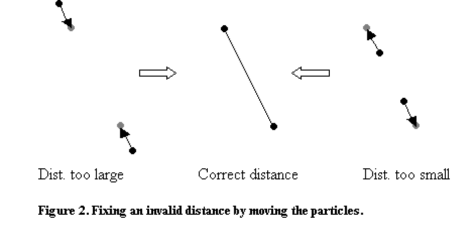
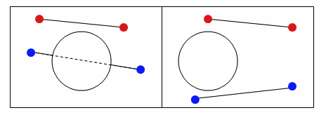
We now extend the experiment to model a stick of length 100. We do this by setting up two individual particles (with positions and ) and then require them to be a distance of 100 apart. Expressed mathematically, we get the following bilateral (equality) constraint:
Although the particles might be correctly placed initially, after one integration step the separation distance between them might have become invalid. In order to obtain the correct distance once again, we move the particles by projecting them onto the set of solutions described by (C2). This is done by pushing the particles directly away from each other or by pulling them closer together (depending on whether the erroneous distance is too small or too large). See Figure 2.
Verlet integration
Verlet算法是经典力学(牛顿力学)中的一种最为普遍的积分方法,被广泛运用在分子运动模拟(Molecular Dynamics Simulation),行星运动以及织物变形模拟等领域。Verlet算法要解决的问题是,给定粒子时刻的位置和速度,得到时刻的位置和速度。最简单的方法是前向计算(考虑当前和未来)的速度位移公式,也就是显式欧拉方法,但精度不够,且不稳定。Verlet积分是一种综合过去、现在和未来的计算方法(居中计算),精度为, 稳定度好,且计算复杂度不比显式欧拉方法高多少。
1 | // Pseudo-code to satisfy (C2) |
2 | delta = x2-x1; |
3 | deltalength = sqrt(delta*delta); |
4 | |
5 | diff = (deltalength-restlength)/deltalength; |
6 | |
7 | x1 += delta*0.5*diff; |
8 | x2 -= delta*0.5*diff; |
Note that delta is a vector so delta*delta is actually a dot product. With restlength=100 the above pseudo-code will push apart or pull together the particles such that they once more attain the correct distance of 100 between them. Again we may think of the situation as if a very stiff spring with rest length 100 has been inserted between the particles such that they are instantly placed correctly.
Now assume that we still want the particles to satisfy the cube constraints. By satisfying the stick constraint, however, we may have invalidated one or more of the cube constraints by pushing a particle out of the cube. This situation can be remedied by immediately projecting the offending particle position back onto the cube surface once more – but then we end up invalidating the stick constraint again.
Really, what we should do is solve for all constraints at once, both (C1) and (C2). This would be a matter of solving a system of equations. However, we choose to proceed indirectly by local iteration. We simply repeat the two pieces of pseudo-code a number of times after each other in the hope that the result is useful. This yields the following code:
1 | // Implements simulation of a stick in a box |
2 | void ParticleSystem::SatisfyConstraints() { |
3 | for(int j=0; j<NUM_ITERATIONS; j++) { |
4 | // First satisfy (C1) |
5 | for(int i=0; i<NUM_PARTICLES; i++) { // For all particles |
6 | Vector3& x = m_x[i]; |
7 | x = vmin(vmax(x, Vector3(0,0,0)), |
8 | Vector3(1000,1000,1000)); |
9 | } |
10 | |
11 | // Then satisfy (C2) |
12 | Vector3& x1 = m_x[0]; |
13 | Vector3& x2 = m_x[1]; |
14 | |
15 | Vector3 delta = x2-x1; |
16 | |
17 | float deltalength = sqrt(delta*delta); |
18 | float diff = (deltalength-restlength)/deltalength; |
19 | |
20 | x1 += delta*0.5*diff; |
21 | x2 -= delta*0.5*diff; |
22 | } |
23 | } |
(Initialization of the two particles has been omitted.) While this approach of pure repetition might appear somewhat naïve, it turns out that it actually converges to the solution that we are looking for! The method is called relaxation (or Jacobi or Gauss-Seidel iteration depending on how you do it exactly, see [Press]). It works by consecutively satisfying various local constraints and then repeating; if the conditions are right, this will converge to a global configuration that satisfies all constraints at the same time. It is useful in many other situations where several interdependent constraints have to be satisfied at the same time.
The number of necessary iterations varies depending on the physical system simulated and the amount of motion. It can be made adaptive by measuring the change from last iteration. If we stop the iterations early, the result might not end up being quite valid but because of the Verlet scheme, in next frame it will probably be better, next frame even more so etc. This means that stopping early will not ruin everything although the resulting animation might appear somewhat sloppier.
Cloth simulation
The fact that a stick constraint can be thought of as a really hard spring should make apparent its usefulness for cloth simulation as sketched in the beginning of this section. Assume, for example, that a hexagonal mesh of triangles describing the cloth has been constructed. For each vertex a particle is initialized and for each edge a stick constraint between the two corresponding particles is initialized (with the constraint’s “rest length” simply being the initial distance between the two vertices).
The function HandleConstraints() then uses relaxation over all constraints. The relaxation loop could be iterated several times. However, to obtain nicely looking animation, actually for most pieces of cloth only one iteration is necessary! This means that the time usage in the cloth simulation depends mostly on the N square root operations and the N divisions performed (where N denotes the number of edges in the cloth mesh). As we shall see, a clever trick makes it possible to reduce this to N divisions per frame update – this is really fast and one might argue that it probably can’t get much faster.
1 | |
2 | // Implements cloth simulation |
3 | struct Constraint { |
4 | int particleA, particleB; |
5 | float restlength; |
6 | }; |
7 | |
8 | // Assume that an array of constraints, m_constraints, exists |
9 | void ParticleSystem::SatisfyConstraints() { |
10 | for(int j=0; j<NUM_ITERATIONS; j++) { |
11 | for(int i=0; i<NUM_CONSTRAINTS; i++) { |
12 | Constraint& c = m_constraints[i]; |
13 | Vector3& x1 = m_x[c.particleA]; |
14 | Vector3& x2 = m_x[c.particleB]; |
15 | |
16 | Vector3 delta = x2-x1; |
17 | float deltalength = sqrt(delta*delta); |
18 | float diff=(deltalength-c.restlength)/deltalength; |
19 | x1 += delta*0.5*diff; |
20 | x2 -= delta*0.5*diff; |
21 | } |
22 | // Constrain one particle of the cloth to origo |
23 | m_x[0] = Vector3(0,0,0); |
24 | } |
25 | } |
We now discuss how to get rid of the square root operation. If the constraints are all satisfied (which they should be at least almost), we already know what the result of the square root operation in a particular constraint expression ought to be, namely the rest length of the corresponding stick. We can use this fact to approximate the square root function. Mathematically, what we do is approximate the square root function by its 1st order Taylor-expansion at a neighborhood of the squared rest length (this is equivalent to one Newton-Raphson iteration with initial guess r). After some rewriting, we obtain the following pseudo-code:
1 | // Pseudo-code for satisfying (C2) using sqrt approximation |
2 | delta = x2-x1; |
3 | delta*=restlength*restlength/(delta*delta+restlength*restlength)-0.5; |
4 | x1 += delta; |
5 | x2 -= delta; |
Notice that if the distance is already correct (that is, if |delta|=restlength), then one gets delta=(0,0,0) and no change is going to happen.
Per constraint we now use zero square roots, one division only, and the squared value restlength*restlength can even be precalculated! The usage of time consuming operations is now down to N divisions per frame (and the corresponding memory accesses) – it can’t be done much faster than that and the result even looks quite nice. Actually, in Hitman, the overall speed of the cloth simulation was limited mostly by how many triangles it was possible to push through the rendering system.
The constraints are not guaranteed to be satisfied after one iteration only, but because of the Verlet integration scheme, the system will quickly converge to the correct state over some frames. In fact, using only one iteration and approximating the square root removes the stiffness that appears otherwise when the sticks are perfectly stiff.
By placing support sticks between strategically chosen couples of vertices sharing a neighbor, the cloth algorithm can be extended to simulate plants. Again, in Hitman only one pass through the relaxation loop was enough (in fact, the low number gave the plants exactly the right amount of bending behavior).
The code and the equations covered in this section assume that all particles have identical mass. Of course, it is possible to model particles with different masses, the equations only get a little more complex.
To satisfy (C2) while respecting particle masses, use the following code:
1 | // Pseudo-code to satisfy (C2) |
2 | delta = x2-x1; |
3 | deltalength = sqrt(delta*delta); |
4 | diff = (deltalength-restlength)/(deltalength*(invmass1+invmass2)); |
5 | x1 += invmass1*delta*diff; |
6 | x2 -= invmass2*delta*diff; |
Here invmass1 and invmass2 are the numerical inverses of the two masses. If we want a particle to be immovable, simply set invmass=0 for that particle (corresponding to an infinite mass). Of course in the above case, the square root can also be approximated for a speed-up.
Rigid bodies
Articulated bodies
Comments and Notes
Conclusion
This paper has described how a physics system was implemented in Hitman. The underlying philosophy of combining iterative methods with a stable integrator has proven to be successful and useful for implementation in computer games. Most notably, the unified particle-based framework, which handles both collisions and contact, and the ability to trade off speed vs. accuracy without accumulating visually obvious errors are powerful features. Naturally, there are still many specifics that can be improved upon. In particular, the tetrahedron model for rigid bodies needs some work. This is in the works.
Verlet算法简要介绍
-
将 和 进行泰勒展开
![]()
-
将以上两个表达式进行相加,得到位置表达式
![]()
-
将1中的两个式子相减,再同时除以 即可获得速度表达式
![]()
这个式子显明,只有在知道前一时刻和后一时刻的位置时,才有可能知道当前时刻的速度。也就是说,在当前时刻不能获得速度信息,必须要等到下一时刻的位置确定以后,才能返回来计算当前的速度。 -
力(加速度)根据当前的位置 ,基于一定的势函数进行更新

Verlet算法积分步运行过程
根据verlet算法,要计算时刻的位置,必须知道 时刻和 时刻的位置, 的速度和 时刻的加速度。具体演绎过程如下:
-
根据 和 时刻的位置、 时刻的加速度 ,获得当前时刻 的位置。
-
根据当前时刻 的位置,更新当前位置下的加速度(受力)。
-
同时,可以更新 时刻的速度。(速度是附带更新了,不更新速度并不妨碍积分过程继续下去。)
那么,现在就获得了 时刻的位置, 时刻的速度和 时刻的加速度,相当于将已知条件向前推进了一步(可以对比引用的部分)。
接下来的过程就是重复上面的过程。下图生动的反映了这个过程。
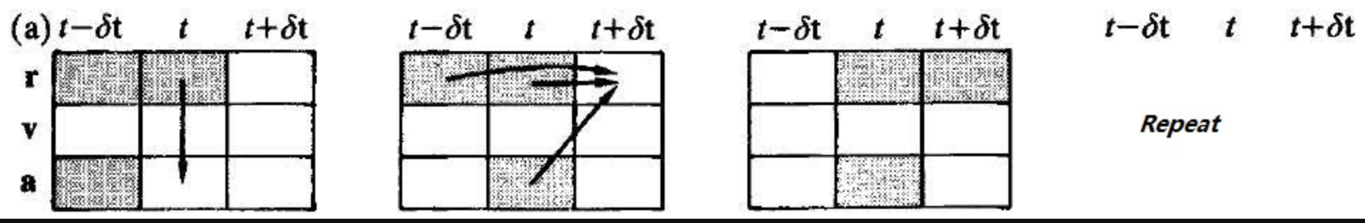
其中表示时间,表示位置,表示速度,表示加速度。
Cloth Simulation using Mass-Spring System
Mass-Spring System
we consider the cloth as a collection of particles interconnected with three types of springs:
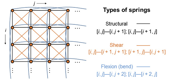
The rest of this section details this mass-spring system.
Particles
We assume the cloth contains (evenly spaced) particles and use (where ) to denote the particle located at the -th row and -th column. Each particle has the following states:
- Mass m (we assume all particles to have identical masses).
- Position .
- Velocity which equals the derivate of with respect to t: = .
The position and velocity of a particle are affected by various types of forces (see Section 1.3). In particular, assuming the accumulated force acting on particle at time to be , then Newton’s second law of motion tells us that the acceleration of this particle at time equals
Springs
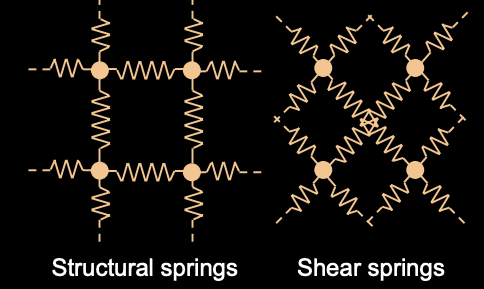
There are three types of springs connecting all particles: structural, shear, and flexion (bend).
- Structural: each particle is connected to (up to) four particles via structural connections: .
- Shear: each particle is connected to (up to) four particles via shear connections: .
- Flexion: each particle is connected to (up to) four particles via flexion connections: .
Thus, each particle can have up to 12 directly connected neighbors.
Stiffness: in this project, we assume all structural springs to have stiffness , shear springs , and flexion strings .
Rest length: generally, a piece of cloth is considered to be in its rest state when there is no deformation (caused by stretching, shearing, or bending). In this project, the original shape of the cloth is a rectangle of size . It follows that the rest lengths for all structural, shear, and flexion springs are , , and , respectively.
Forces
There are four types of forces you will need to consider for this project:
- Spring forces: given spring connecting two particles located at and with stiffness and rest length , the spring force acting on equals
This force changes over time as the particles move.
- Gravity: each particle is affected by (simple) gravity given by
where . Notice that in this project, the “up” direction is the Y-axis (i.e., ), NOT the Z-axis. This force stays constant over time.
-
Damping: for a particle with velocity , the amount of damping force it receives equals where is a constant. This force changes over time as changes.
-
Viscous fluid: to handle a cloth’s viscous behavior, we assume each particle with velocity is pushed by an imaginary viscous fluid with
where is the surface normal at the particle’s location, is a constant, and is a constant vector specifying the velocity of the viscous fluid. This force changes over time.
Animating the System
As mentioned in class, animating a mass-spring system involves solving an initial value problem. In particular, for each particle you are given its mass (which stays constant for all particles), initial position and velocity . Given , you need to use Euler’s method to compute the position and velocity of each particle at time-steps
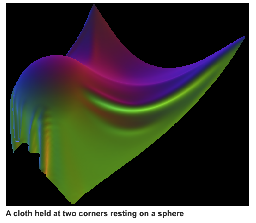
You need to pin two particles and , which correspond to the upper left and right corners of the cloth. That is, the positions of these particles are fixed to their inital values. If no particle is pinned in place, the entire cloth will undergo a never-ending free fall because of gravity!
Global Variables
A number of global variables are used to store various mass-spring system configurations and particle states.
Constants (time-invariant):
- meshResolution stores the integer which determines the total number of particles (see Section 1.1).
- mass stores the mass for every particle.
- K is a vec3 where , , and indicate the stiffnesses of all structural, shear, and flexion springs, respectively.
- Similarly, restLength is a vec3 where , , and gives the rest lengths of structural, shear, and flexion springs, respectively.
- stores the coefficient used for computing damping forces .
- and respectively store the coefficient and the vector used for computing viscous forces .
All the time-invariant constants have been handled by the provided code. You can directly access them in your code.
Particle states (time-variant):
- vertexPosition and vertexVelocity are two arrays storing the position and velocity of each particle, respectively. You will need to update them in a step-by-step manner (see Section 2.2 for details).
- vertexNormal stores surface normal directions at each particle (which is needed for rendering as well as computing ). You do NOT have to modify this array: the provided code automatically changes vertex normals based on the updated positions.
Global Functions
A number of getter & setter functions are provided for your convenience:
- getPosition(i, j) returns the position of particle [i,j] as a vec3.
- setPosition(i, j, x) sets the position of particle [i,j] to x.
- getNormal(i, j) returns the surface normal at particle [i,j] as a vec3.
- getVelocity(i, j) returns the velocity of particle [i,j] as a vec3.
- setVelocity(i, j, v) sets the position of particle [i,j] to v.
Function(Simulate) to Complete
Finish the key function simulate() to animate the cloth.
This function takes one parameter stepSize (i.e, Δt) and performs ONE iteration of Euler’s method. Precisely, assuming vertexPosition and vertexVelocity currently stores the position and velocity for each particle at time . After executing simulate() once, vertexPosition and vertexVelocity should be updated so that they store and , respectively.
To achieve this, we will need to do the following:
- Compute the accumulated force acting on each particle [i,j] for i,j∈{0,1,…,n−1} based on each particle’s current position and velocity.
- Update the velocity of each particle using
- Update the position of each particle (except for the two pinned ones which stay static) using
Notice that the updated velocity (from Step 2) is used here for better numerical stability.
With simulate() properly implemented, we should see the cloth deforming.
Cloth Theoris
Cloth is a very interesting and complicated subject in computer graphics. More accurately referred to as thin-shell material models, the objective is to simulate the motion of thin objects such as cloth, folded paper, clothing, etc. People have come up with a wide array of cloth models, and no single model has proven itself strongly dominant. In order to compare the existing models, we’ll break down the model into five categories:
- equations of motion
- integrators
- collisions
- improvements
- rendering
Equations of Motion
#####Mass-Spring Model
The equations of motion for a system govern the motion of the system. One of the first (and simplest) cloth models is as follows: consider the sheet of cloth. Divide it up into a series of approximately evenly spaced masses M. Connect nearby masses by a spring, and use Hooke’s Law and Newton’s 2nd Law as the equations of motion. Various additions, such as spring damping or angular springs, can be made. A mesh structure proves invaluable for storing the cloth and performing the simulation directly on it. Each vertex can store all of its own local information (velocity, position, forces, etc.) and when it comes time to render, the face information allows for immediate rendering as a normal mesh.
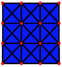
In the cloth structure seen above, the red nodes are vertices, and the black lines are springs. The diagonal springs are necessary to resist collapse of the face; it ensures that the entire cloth does not decompose into a straight line. The blue represents the mesh faces. Looking at the equations of motion:
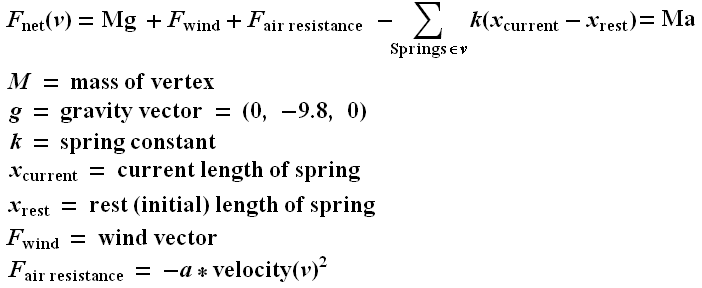
To determine M, a simple constant (say, 1) is fine for all vertices. To be more accurate, you should compute the area of each triangle, and assign 1/3rd of it towards the mass of each incident vertex; this way the mass of the entire cloth is the total area of all the triangles times the mass density of the cloth. The gravity vector can also be an arbitrary vector; if all distance units were meters, time was measured in seconds, and we were on the surface of the earth and “y” was the “up/down” vector, (0, -9.8, 0) would be the correct “g”. X(current) is just the current length of the spring, and X(rest), the spring’s rest length, needs to be stored in each spring structure. F(wind) can just be some globally varying constant function, say (sin(xyt), cos(zt), sin(cos(5xyz)). a is a simple constant determined by the properties of the surrounding fluid (usually air,) but it can also be used to achieve certain cloth effects, and can help with the numeric stability of the cloth. k is a very important constant; if too low, the cloth will sag unrealistically:
On the other hand, if k is chosen too large, the system will be unrealistically tight (retain its original shape.) Worse yet, the system will be more and more “stiff” the larger k is chosen; this is a mathematical term for explosive. Without careful attention to the integration method, the system will gain energy as a function of time, and the system will explode with vertices tending towards infinity.
Elasticity Model
The mass-spring model above has several shortcommings. Mostly, it is not very physically correct, so attempting to use physically accurate constants is generally unsuccessful. Furthermore it requires guessing arbitrarily which vertices should be connected to which by a spring, and choosing k such that increasing the resolution of the grid leads to a system with similar characteristics can be tricky. A more accurate model, based on integrating an energy over the surface of the cloth, consider energy terms such as:
- Triangles and edges resist changes in their size, and compressing or expanding them requires energy
- Edges resist bending, so bending the two faces adjacent away from the inital bend of this edge (0 for a planar initial condition) requires energy
- Triangles resist deformation (in addition to resisting changes in size.) So attempting to shear or otherwise deform a triangle requires energy
We imagine a giant vector, S, representing every important variable in the system (position and velocities of all the vertices, although potentially there could be more degrees of freedom.) Given energy as a function of the current state of the system, E(S), the equation of motion for a single vertex at position (x, y, z) is then rather simple:
Evaluating this, however, is not so simple. Generally this derivative must be computed analytically. Suppose we attempted to compute the derivative numerically; we consider the state variable constant, reducing our energy E(s) to E(x). We then say:
But evaluating the energy E(S) takes a long time; we must iterate over all the vertices, faces, and edges, summing the energy of each one. But we might notice that the effect of x on the energy depends on a very local region (all the incident edges and faces, called the one-ring of the vertex.) So to keep our algorithm O(n) when doing the derivative numerically, we must make sure that we compute E(x) by only considering the energy of the one-ring of the vertex in question.
In general, this method can be very challenging to implement, and although it is physically much more sound, in practice the results are in some ways better and in some ways worse than the mass-spring model. This method of cloth animation, including the derivation of the energy terms, is discussed thoroughly in paper Large Steps in Cloth Simulation
Integrators
After we decide on the cloth model, we need a method to integrate the equation of motion. Assuming our model is newtonian, we have at every vertex defined a position and velocity at each time step t, and our equation of motion tells us dv/dt, or the acceleration of each vertex at time t, and we want to know the position and velocity at the next time step.
Euler’s Method (Explicit)
The simplest method for integrating our equations is Euler’s method. It goes like this:
The t subscript on dv/dt means “dv/dt evaluated at time t” (as opposed to say, dv/dt at the previous or the next time step.) Delta t refers to the timestep we’re taking (smaller time step means more accurate results but slower computation times.) We can derive the above method quite simply:
And likewise for the velocity term. This method is very simple to implement, but it has the disadvantage that for most systems, it has a large amount of positive feedback, and tends to cause all variables to rapidly increase to ridiculous values, no matter how small the time step. This explosive behavior is characteristic of all explicit integrators; the term explicit just means that the state at (t+1) is evaluated by just considering the state at time (t). The explosive behavior is arguably the most frustrating aspect of all simulations, and a lot of work goes into dealing with this problem. In cloth, the first way around this is to put enough damping in the system (spring damping, air resistance, velocity damping, etc.) that in a single time step energy decreases the naturally, and the feedback will never occur. Another way is to use one of a vast array of add-ons to the cloth model (discussed later) that prevent the explosive behavior. The only way to solve this problem without altering the model is to use an implicit integrator.
Runge Kutta (Explicit)
Euler’s method is not only explosive, it is very inaccurate. As you decrease the time step, the error decreases proportionally. It is possible to use higher-order terms of the derivative to create a much more accurate integrator. There are many such methods, one of the most widely-used of which is called Runge-Kutta. The N-th order Runge-kutta algorithm considers derivative terms up to the N-th order. For various reasons, 4th order is considered optimal, since it gurantees the integrator error decreases proportional to the fourth power of the time step (and it is not true that 5-th order is proportional to the fifth power of the time step.) The algorithm is also excellent because it still only needs the first derivative; higher derivatives are efficently computed numerically just by knowing how to compute the first derivative. While very accurate, it takes slightly longer to compute, and still suffers from all the problems of explicit models, so even if it takes the system longer to explode, in general it still will.
Verlet Algorithm (Explicit)
The Verlet integration algorithm is such an explicit model with the very interesting propety that it does not need to know anything about the velocity; it computes this internally via looking at the position at both the current and previous time step.
Another wonderful aspect of this algorithm is that like 4th order Runge-Kutta, it is 4th order accurate. Because it is quite accurate, easy to implement, and does not need the velocity terms, it is my favorite explicit model and the one I use in all my cloth models.
Euler’s Method (Implicit)
Unlike an explicit integrator, an implicit integrator uses the state variable at the current time step and the derivative at the next time step to compute the state variable at the next time step. There is a perfect implicit analogy to Euler’s method; in our model, we have the following equations:
The only change is the subscript from “t” to “t + dt”. We notice quickly that we only need to deal with the v(t+1) term; the x(t+1) term can then be trivially computed using this new velocity. But computing this new velocity can be extremely tricky. In either the mass-spring or elasticity model, this requires the following: consider the big state vector S (all the velocities and positions in the system) as a 6n x 1 matrix (where n is the number of vertices. Linearize the equations of motion so we can represent dv/dt at time t as follows:
Where Q is a giant 3n by 6n matrix representing the linear relationship between the change in velocities and the state of the system. We would then substitute this into the implicit euler equation for dv/dt, and solve for the velocity at the new time step. However, this would involve inverting the massive matrix Q (which is thankfully very sparse, assuming not every vertex is connected to every other vertex.) This is generally accomplished with linear conjugate gradient descent. If you’re interested in implementing this, see this paper (the same paper as above.) Overall, this algorithm is very complicated to implement for cloth models, but because of the negative feedback, the energy in the system tends to decrease, rather than increase explosively. This enables you to take much larger time steps and remain stable, and avoids the necessity of excessive damping terms. However, it is very time consuming to take each time step, requires convergence of a matrix inversion algorithm, and because such large time steps are taken and the relationship between error and time step is linear (as with Explicit Euler’s,) the algorithm is a very bad approximation of the underlying motion we are integrating.
Higher order implicit algorithms
One might expect that there is an implicit analogy to Runge-Kutta. While such an analogy exists, and has both the advantage of good errors and a stable system, I have never seen it applied to cloth models; the 1st-order implicit version is sufficently complicated for anyone.
Symplectic Euler’s Method (Semi-Implicit)
Many algorithms exist which are compromises between implicit and explicit models. A simple one is called Symplectic Euler’s Method. It’s equation of motion is:
It is called semi-implicit because it computes the velocity explicitly, but the new position implicitly. This helps reduce the feedback (positive or negative) and can greatly improve stability, at no cost in algorithmic complexity. It also has the powerful advantage that in many systems it conserves energy on average. However, it does not conserve phase or oscillatory motion: in cloth, this results in strange out-of-phase circulations occurring all over the mesh, so in general this algorithm is not a good choice for cloth. Higher order symplectic models exist, but they have similar properties, except for the higher order accuracy.
Collisions
There is no avoiding it; collisions are very hard to deal with when it comes to cloth. Doing it in a physically accurate manner is a complete nightmare, and I have never read a paper that claims to have implemented this. Hacking up a solution with even reasonably plausible results is challenging enough; making gurantees about the cloth not interescting itself or not intersecting other objects is also challenging, but some papers propose complicated models that claim to have this propety; certainly, they have very visually pleasing results. To approach the collision problem, we break it down into two types: cloth-cloth, and cloth-object.
Cloth-Object Collisions
Generally the easier of the two types of collisions to deal with, we assume we have some solid objects in the scene, and independent of their motion, their position at and around time t is fixed and known. These objects might be represented as geometric primitives (cylinders, spheres, cubes, etc.) or the interior of a mesh.
Physically Correct Model
The physically correct method of cloth-object collisions is as follows:
- Starting at time t and cloth positions x(t), compute the proposed x(t + dt)
- For every face on the mesh, consider its initial and final position. If between t and t + dt, this face has interacted an external object, compute the exact time when these surfaces first came into contact. If the face was previously in contact with a surface, and it is no longer in contact, disconnect the surfaces.
- Find the time of the earliest such collision. Back the simulation up to this time, and mark this face as being in contact with the surface it hit. When a face is marked as in contact, we need to compute all of its static and kinetic friction forces - this requires correctly handling the normal vectors of the contact surfaces.
- Resume the simulation from this new time step, and repeat.
This algorithm is extremely annoying to implement and slow, because we will end up creeping along very slowly as we have to keep stepping forward, noticing a collision, backing up, and repeating. Adaptive time stepping doesn’t even help, since we have no choice but to make small time steps all the time. While some papers claim to deal with the friction forces correctly, almost all of them refuse to back the system up, instead making some best guess as to the correct location of the face.
Easy-to-implement Model
In practice the above is very annoying; even detecting the collision can be frustrating since the path taken inbetween the two time steps is a prism-like volume. The model I use is considerably more problematic but reasonable to implement. Firstly, we do not deal with faces or edges at all, and we do not deal with the intermediate time steps; any of the cases below will be missed by my algorithm (red = initial position, blue = new position.)
The only thing my algorithm considers is if a vertex at the positions computed for the next time step is inside one of the objects in the scene, we detect a collision. Our response can be one of two things: move the vertex back to where it came from (this is equivalent to an infinite-friction surface) or we could “repel” the object in some fashion. Given a position, many objects have a natural point on the surface associated with it. Take for example a sphere; given a position, consider the intersection of the sphere with the line from the sphere’s center to this position. This point is the closest point on the surface associated with the input point, and while such a position is well defined for all objects, it is especially easy to compute in the case of simple geometric objects. If, rather than moving a point back to its original location we move it to its “repelled” point, we will give the visual apperance of a very slippery (almost zero friction) surface. In the limit as our cloth is refined, with more and more vertices and smaller and smaller faces, the fact that we consider only vertices will be irrelivant, and this model will perform reasonably well.
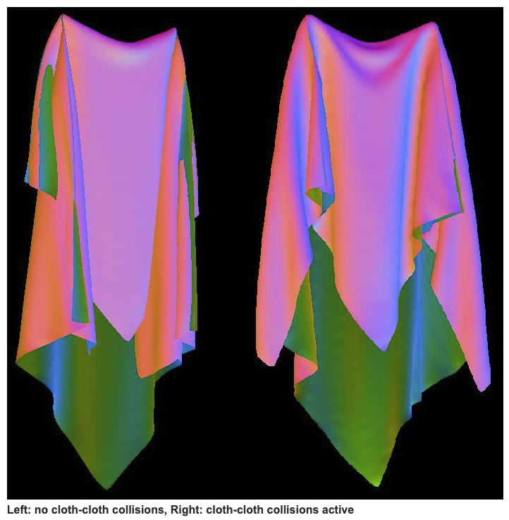
Cloth-Cloth Collisions
Cloth looks very unrealistic if it passes through itself. A simple solution is as follows: if two regions of the cloth are too close to each other, apply a repulsive force to the vertices around this region, encouraging seperation. This is very ugly, in practice, since it is very sensitive to the definition of “too close”, the choice of time step, the choice of the repulsive forces, and can further contribute to numeric instability. Despite all of these problems, it is what this paper does. I don’t like this method and have never implemented it.
A seperate, powerful solution is as follows: compute the new positions and determine any intersections that happened. Now go back to the previous time step, and modify the magnitudes of the velocities in such a way that the collisions no longer occur. This is both not too hard to implement, effective in practice, and can gurantee that no collisions occur. However, determining all the collisions is very time consuming and greatly slows down the algorithm, in addition to causing a geometric headache. So the algorithm I use is different from both of these approaches.
My algorithm considers the cloth as a set of connected marbles. We imagine a virtual marble to be centered around each vertex. Marbles are not considered to be touching if their associated vertices are connected by a spring; thus, we can set the radius of a marble larger than the distance between two vertices. If we do this, then we have covered the entire surface of the cloth, and if no two marbles pass through each other between t and t + dt, the cloth has not intersected itself. The update algorithm is very simple: if the new positions contain vertices whose marbles are inside each other (the distance between the vertices is less than twice the marble radius,) back the vertices up such that this collision has no occured (although we remain at the new time step.) We can make several choices about the velocities; generally it is simplest to zero the new velocities, although it is possible to get “bouncing off” effects if desired. In general this algorithm works well and in my opinion is the easiest to implement.
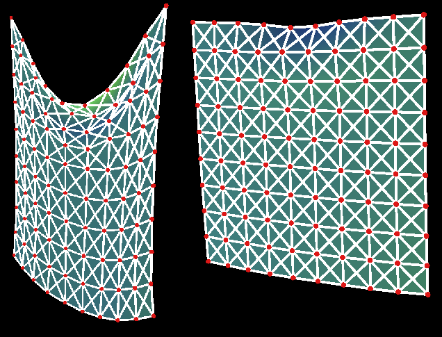
Suppose we start with a planar cloth and fix two arbitrary vertices in the middle of the cloth. Without cloth-cloth collisions, the cloth will settle into a position where it is highly self-intsersecting, but with the cloth-cloth collision algorithm above we avoid this interpenetration and get very convincing cloth-like folds.
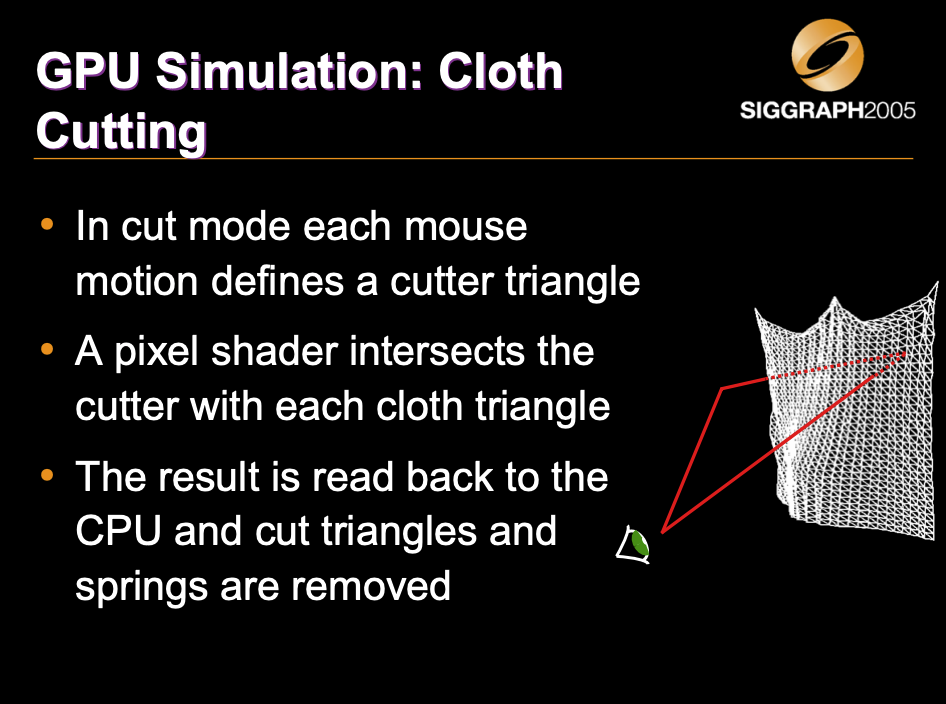
Cloth Simulation on the GPU Cloth Simulation on the GPU
A method to simulate cloth on any GPU
- Takes advantage of the massive parallel computation horsepower of GPUs
- Geared toward performance and visual realism, not physical accuracy
- Suitable to 3D games and virtual reality systems
Cloth as a Set of Particles
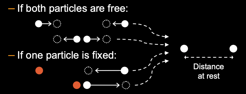
- Each particle is subject to
– A force (gravity, wind, drag, etc.)
– Various constraints:
• To maintain overall shape (springs)
• To prevent interpenetration with the environment - Constraints are resolved by relaxation
- CPU version successfully used in games:
Jakobsen, T. “Advanced character physics”, GDC 01
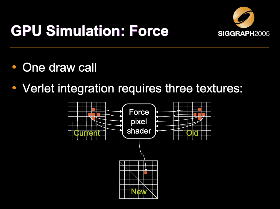
Force
- Verlet integration:
• Δt: simulation time step
• P(t): particle position
• F(t): force
• k: damping coefficient
- No force applied to fixed or user-moved particles
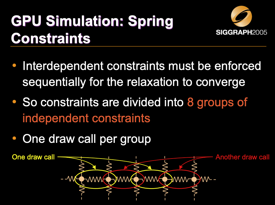
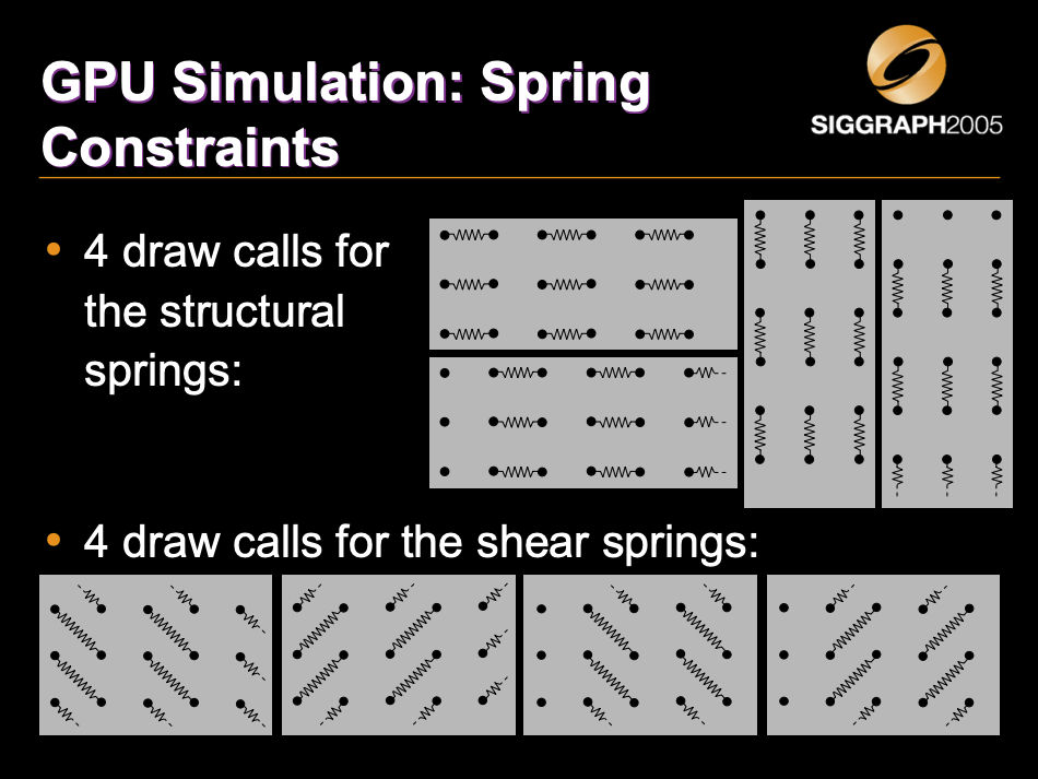
Spring Constraints
- Particles are linked by springs:
![]()
- A spring is simulated as a distance constraint between two particles
Distance Constraint
A distance constraint between two particles is enforced by moving them away or towards each other:
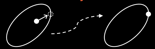
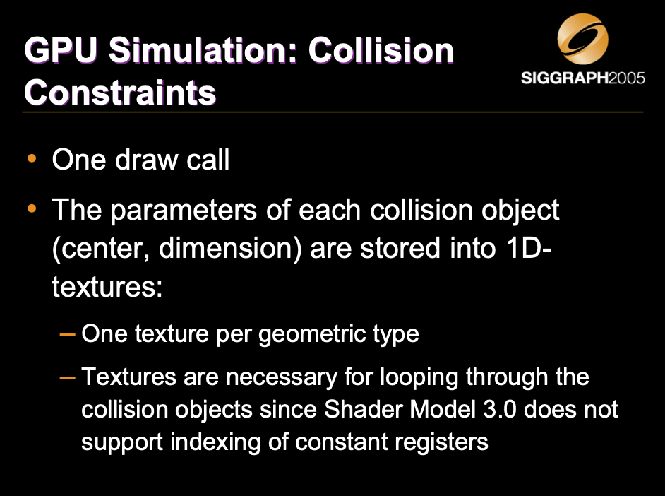
Collision Constraints Collision Constraints
- The environment is defined as a set of collision objects (planes, spheres, boxes,
ellipsoids) - A collision constraint between a particle and a collision object is enforced by moving the
particle outside the object:
![]()
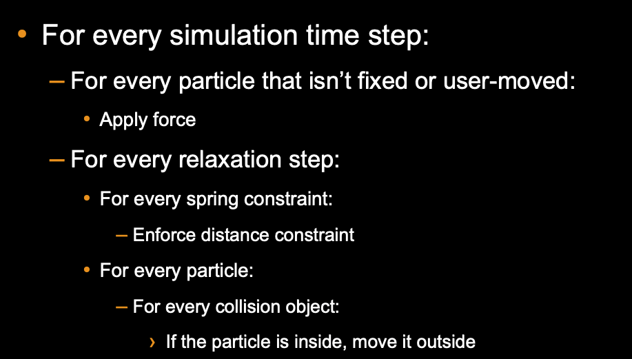
Algorithm Outline Algorithm Outline
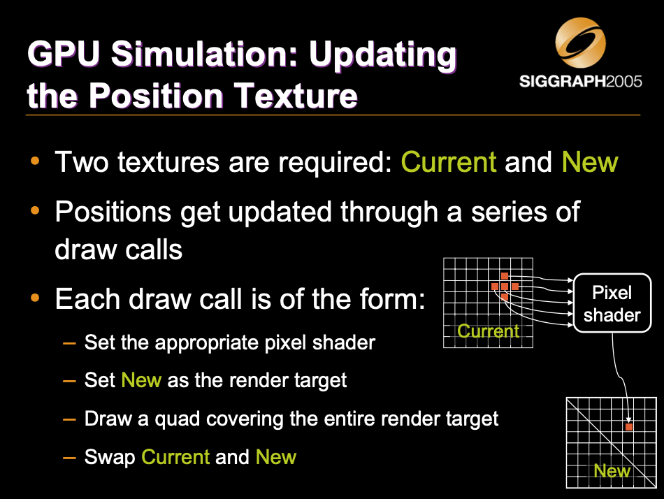
GPU Implementation Overview
- The particle positions and normals are stored into floating-point textures
- The CPU never reads back these textures!
- At every frame:
– GPU simulation: Update the position and normal textures
– GPU rendering: Render using vertex texture fetch (available on Shader Model 3.0 and above)
Fluid Simulation
Chapter 38. Fast Fluid Dynamics Simulation on the GPU
This chapter describes a method for fast, stable fluid simulation that runs entirely on the GPU. It introduces fluid dynamics and the associated mathematics, and it describes in detail the techniques to perform the simulation on the GPU. After reading this chapter, you should have a basic understanding of fluid dynamics and know how to simulate fluids using the GPU. The source code accompanying this book demonstrates the techniques described in this chapter.
1 Introduction
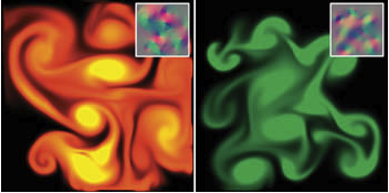
Fluids are everywhere: water passing between riverbanks, smoke curling from a glowing cigarette, steam rushing from a teapot, water vapor forming into clouds, and paint being mixed in a can. Underlying all of them is the flow of fluids. All are phenomena that we would like to portray realistically in interactive graphics applications. Figure 38-1 shows examples of fluids simulated using the source code provided with this book.
Fluid simulation is a useful building block that is the basis for simulating a variety of natural phenomena. Because of the large amount of parallelism in graphics hardware, the simulation we describe runs significantly faster on the GPU than on the CPU. Using an NVIDIA GeForce FX, we have achieved a speedup of up to six times over an equivalent CPU simulation.
1.1 Our Goal
Our goal is to assist you in learning a powerful tool, not just to teach you a new trick. Fluid dynamics is such a useful component of more complex simulations that treating it as a black box would be a mistake. Without understanding the basic physics and mathematics of fluids, using and extending the algorithms we present would be very difficult. For this reason, we did not skimp on the mathematics here. As a result, this chapter contains many potentially daunting equations. Wherever possible, we provide clear explanations and draw connections between the math and its implementation.
1.2 Our Assumptions
The reader is expected to have at least a college-level calculus background, including a basic grasp of differential equations. An understanding of vector calculus principles is helpful, but not required (we will review what we need). Also, experience with finite difference approximations of derivatives is useful. If you have ever implemented any sort of physical simulation, such as projectile motion or rigid body dynamics, many of the concepts we use will be familiar.
#####1.3 Our Approach
The techniques we describe are based on the “stable fluids” method of Stam 1999. However, while Stam’s simulations used a CPU implementation, we choose to implement ours on graphics hardware because GPUs are well suited to the type of computations required by fluid simulation. The simulation we describe is performed on a grid of cells. Programmable GPUs are optimized for performing computations on pixels, which we can consider to be a grid of cells. GPUs achieve high performance through parallelism: they are capable of processing multiple vertices and pixels simultaneously. They are also optimized to perform multiple texture lookups per cycle. Because our simulation grids are stored in textures, this speed and parallelism is just what we need.
This chapter cannot teach you everything about fluid dynamics. The scope of the simulation concepts that we can cover here is necessarily limited. We restrict ourselves to simulation of a continuous volume of fluid on a two-dimensional rectangular domain. Also, we do not simulate free surface boundaries between fluids, such as the interface between sloshing water and air. There are many extensions to these basic techniques. We mention a few of these at the end of the chapter, and we provide pointers to further reading about them.
We use consistent mathematical notation throughout the chapter. In equations, italics are used for variables that represent scalar quantities, such as pressure, p. Boldface is used to represent vector quantities, such as velocity, u. All vectors in this chapter are assumed to be two-dimensional.
Section 38.2 provides a mathematical background, including a discussion of the equations that govern fluid flow and a review of basic vector calculus concepts and notation. It then discusses the approach to solving the equations. Section 38.3 describes implementation of the fluid simulation on the GPU. Section 38.4 describes some applications of the simulation, Section 38.5 presents extensions, and Section 38.6 concludes the chapter.
2 Mathematical Background
To simulate the behavior of a fluid, we must have a mathematical representation of the state of the fluid at any given time. The most important quantity to represent is the velocity of the fluid, because velocity determines how the fluid moves itself and the things that are in it. The fluid’s velocity varies in both time and space, so we represent it as a vector field.
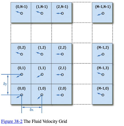
A vector field is a mapping of a vector-valued function onto a parameterized space, such as a Cartesian grid. (Other spatial parameterizations are possible, but for purposes of this chapter we assume a two-dimensional Cartesian grid.) The velocity vector field of our fluid is defined such that for every position , there is an associated velocity at time t, , as shown in Figure 38-2.
The key to fluid simulation is to take steps in time and, at each time step, correctly determine the current velocity field. We can do this by solving a set of equations that describes the evolution of the velocity field over time, under a variety of forces. Once we have the velocity field, we can do interesting things with it, such as using it to move objects, smoke densities, and other quantities that can be displayed in our application.
2.1 The Navier-Stokes Equations for Incompressible Flow
In physics it’s common to make simplifying assumptions when modeling complex phenomena. Fluid simulation is no exception. We assume an incompressible, homogeneous fluid.
A fluid is incompressible if the volume of any subregion of the fluid is constant over time. A fluid is homogeneous if its density, , is constant in space. The combination of incompressibility and homogeneity means that density is constant in both time and space. These assumptions are common in fluid dynamics, and they do not decrease the applicability of the resulting mathematics to the simulation of real fluids, such as water and air.
We simulate fluid dynamics on a regular Cartesian grid with spatial coordinates ${\mathbf x} = (x, y) $and time variable t. The fluid is represented by its velocity field , as described earlier, and a scalar pressure field . These fields vary in both space and time. If the velocity and pressure are known for the initial time , then the state of the fluid over time can be described by the Navier-Stokes equations for incompressible flow:
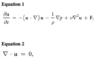
where is the (constant) fluid density, is the kinematic viscosity, and represents any external forces that act on the fluid. Notice that Equation 1 is actually two equations, because is a vector quantity:
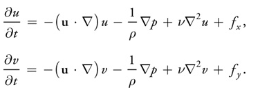
Thus, we have three unknowns (u, v, and p) and three equations.
The Navier-Stokes equations may initially seem daunting, but like many complex concepts, we can better understand them by breaking them into simple pieces. Don’t worry if the individual mathematical operations in the equations don’t make sense yet. First, we will try to understand the different factors influencing the fluid flow. The four terms on the right-hand side of Equation 1 are accelerations. We’ll look at them each in turn.
2.2 Terms in the Navier-Stokes Equations
Advection
The velocity of a fluid causes the fluid to transport objects, densities, and other quantities along with the flow. Imagine squirting dye into a moving fluid. The dye is transported, or advected, along the fluid’s velocity field. In fact, the velocity of a fluid carries itself along just as it carries the dye. The first term on the right-hand side of Equation 1 represents this self-advection of the velocity field and is called the advection term.
Pressure
Because the molecules of a fluid can move around each other, they tend to “squish” and “slosh.” When force is applied to a fluid, it does not instantly propagate through the entire volume. Instead, the molecules close to the force push on those farther away, and pressure builds up. Because pressure is force per unit area, any pressure in the fluid naturally leads to acceleration. (Think of Newton’s second law, F = m a.) The second term, called the pressure term, represents this acceleration.
Diffusion
From experience with real fluids, you know that some fluids are “thicker” than others. For example, molasses and maple syrup flow slowly, but rubbing alcohol flows quickly. We say that thick fluids have a high viscosity. Viscosity is a measure of how resistive a fluid is to flow. This resistance results in diffusion of the momentum (and therefore velocity), so we call the third term the diffusion term.
External Forces
The fourth term encapsulates acceleration due to external forces applied to the fluid. These forces may be either local forces or body forces. Local forces are applied to a specific region of the fluid—for example, the force of a fan blowing air. Body forces, such as the force of gravity, apply evenly to the entire fluid.
We will return to the Navier-Stokes equations after a quick review of vector calculus. For a detailed derivation and more details, we recommend Chorin and Marsden 1993 and Griebel et al. 1998.
2.3 A Brief Review of Vector Calculus
Equations 1 and 2 contain three different uses of the symbol (often pronounced “del”), which is also known as the nabla operator. The three applications of nabla are the gradient, the divergence, and the Laplacian operators, as shown in Table 38-1. The subscripts and used in the expressions in the table refer to discrete locations on a Cartesian grid, and and are the grid spacing in the and dimensions, respectively (see Figure 38-2).
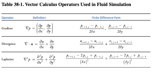
The gradient of a scalar field is a vector of partial derivatives of the scalar field. Divergence, which appears in Equation 2, has an important physical significance. It is the rate at which “density” exits a given region of space. In the Navier-Stokes equations, it is applied to the velocity of the flow, and it measures the net change in velocity across a surface surrounding a small piece of the fluid. Equation 2, the continuity equation, enforces the incompressibility assumption by ensuring that the fluid always has zero divergence. The dot product in the divergence operator results in a sum of partial derivatives (rather than a vector, as with the gradient operator). This means that the divergence operator can be applied only to a vector field, such as the velocity, .
Notice that the gradient of a scalar field is a vector field, and the divergence of a vector field is a scalar field. If the divergence operator is applied to the result of the gradient operator, the result is the Laplacian operator . If the grid cells are square (that is, if , which we assume for the remainder of this chapter), the Laplacian simplifies to:
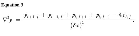
The Laplacian operator appears commonly in physics, most notably in the form of diffusion equations, such as the heat equation. Equations of the form are known as Poisson equations. The case where b = 0 is Laplace’s equation, which is the origin of the Laplacian operator. In Equation 2, the Laplacian is applied to a vector field. This is a notational simplification: the operator is applied separately to each scalar component of the vector field.
2.4 Solving the Navier-Stokes Equations
The Navier-Stokes equations can be solved analytically for only a few simple physical configurations. However, it is possible to use numerical integration techniques to solve them incrementally. Because we are interested in watching the evolution of the flow over time, an incremental numerical solution suits our needs.
As with any algorithm, we must divide the solution of the Navier-Stokes equations into simple steps. The method we use is based on the stable fluids technique described in Stam 1999. In this section we describe the mathematics of each of these steps, and in Section 38.3 we describe their implementation using the Cg language on the GPU.
First we need to transform the equations into a form that is more amenable to numerical solution. Recall that the Navier-Stokes equations are three equations that we can solve for the quantities u, v, and p. However, it is not obvious how to solve them. The following section describes a transformation that leads to a straightforward algorithm.
The Helmholtz-Hodge Decomposition
Basic vector calculus tells us that any vector can be decomposed into a set of basis vector components whose sum is . For example, we commonly represent vectors on a Cartesian grid as a pair of distances along the grid axes: . The same vector can be written , where and are unit basis vectors aligned to the axes of the grid.
In the same way that we can decompose a vector into a sum of vectors, we can also decompose a vector field into a sum of vector fields. Let be the region in space, or in our case the plane, on which our fluid is defined. Let this region have a smooth (that is, differentiable) boundary, , with normal direction . We can use the following theorem, as stated in Chorin and Marsden 1993.
Helmholtz-Hodge Decomposition Theorem
A vector field on can be uniquely decomposed in the form:
Equation 7:
where has zero divergence and is parallel to ; that is, onWe use the theorem without proof. For details and a proof of this theorem, refer to Section 1.3 of Chorin and Marsden 1993.
This theorem states that any vector field can be decomposed into the sum of two other vector fields: a divergence-free vector field, and the gradient of a scalar field. It also says that the divergence-free field goes to zero at the boundary. It is a powerful tool, leading us to two useful realizations.
First Realization
Solving the Navier-Stokes equations involves three computations to update the velocity at each time step: advection, diffusion, and force application. The result is a new velocity field, , with nonzero divergence. But the continuity equation requires that we end each time step with a divergence-free velocity. Fortunately, the Helmholtz-Hodge Decomposition Theorem tells us that the divergence of the velocity can be corrected by subtracting the gradient of the resulting pressure field:
Equation 8
Second Realization
The theorem also leads to a method for computing the pressure field. If we apply the divergence operator to both sides of Equation 7, we obtain:
Equation 9
But since Equation 2 enforces that , this simplifies to:
Equation 10
which is a Poisson equation (see Section 2.3) for the pressure of the fluid, sometimes called the Poisson-pressure equation. This means that after we arrive at our divergent velocity, , we can solve Equation 10 for p, and then use and p to compute the new divergence-free field, , using Equation 8. We’ll return to this later.
Now we need a way to compute . To do this, let’s return to our comparison of vectors and vector fields. From the definition of the dot product, we know that we can find the projection of a vector onto a unit vector by computing the dot product of and . The dot product is a projection operator for vectors that maps a vector onto its component in the direction of . We can use the Helmholtz-Hodge Decomposition Theorem to define a projection operator, , that projects a vector field onto its divergence-free component, . If we apply to Equation 7, we get:
But by the definition of . Therefore, . Now let’s use these ideas to simplify the Navier-Stokes equations.
First, we apply our projection operator to both sides of Equation 1:
Because is divergence-free, so is the derivative on the left-hand side, so Also, , so the pressure term drops out. We’re left with the following equation:
Equation 11
The great thing about this equation is that it symbolically encapsulates our entire algorithm for simulating fluid flow. We first compute what’s inside the parentheses on the right-hand side. From left to right, we compute the advection, diffusion, and force terms. Application of these three steps results in a divergent velocity field, , to which we apply our projection operator to get a new divergence-free field, . To do so, we solve Equation 10 for p, and then subtract the gradient of p from , as in Equation 8.
In a typical implementation, the various components are not computed and added together, as in Equation 11. Instead, the solution is found via composition of transformations on the state; in other words, each component is a step that takes a field as input, and produces a new field as output. We can define an operator that is equivalent to the solution of Equation 11 over a single time step. The operator is defined as the composition of operators for advection ( ), diffusion ( ), force application ( ), and projection ( ):
Equation 12:
Thus, a step of the simulation algorithm can be expressed The operators are applied right to left; first advection, followed by diffusion, force application, and projection. Note that time is omitted here for clarity, but in practice, the time step must be used in the computation of each operator. Now let’s look more closely at the advection and diffusion steps, and then approach the solution of Poisson equations.
Advection
Advection is the process by which a fluid’s velocity transports itself and other quantities in the fluid. To compute the advection of a quantity, we must update the quantity at each grid point. Because we are computing how a quantity moves along the velocity field, it helps to imagine that each grid cell is represented by a particle. A first attempt at computing the result of advection might be to update the grid as we would update a particle system. Just move the position, , of each particle forward along the velocity field the distance it would travel in time t:
You might recognize this as Euler’s method; it is a simple method for explicit (or forward) integration of ordinary differential equations. (There are more accurate methods, such as the midpoint method and the Runge-Kutta methods.)
There are two problems with this approach:
- **The first is that simulations that use explicit methods for advection are unstable for large time steps, and they can “blow up” if the magnitude of u(t)t is greater than the size of a single grid cell. **
- The second problem is specific to GPU implementation.
We implement our simulation in fragment programs, which cannot change the locations of the fragments they are writing. This forward-integration method requires the ability to “move” the particles, so it cannot be implemented on current GPUs.
The solution is to invert the problem and use an implicit method (Stam 1999). Rather than advecting quantities by computing where a particle moves over the current time step, we trace the trajectory of the particle from each grid cell back in time to its former position, and we copy the quantities at that position to the starting grid cell. To update a quantity q (this could be velocity, density, temperature, or any quantity carried by the fluid), we use the following equation:
Equation 13
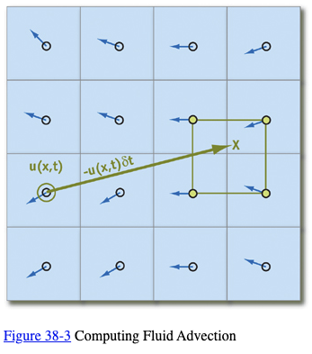
Not only can we easily implement this method on the GPU, but as Stam showed, it is stable for arbitrary time steps and velocities. Figure 38-3 depicts the advection computation at the cell marked with a double circle. Tracing the velocity field back in time leads to the green x. The four grid values nearest the green x (connected by a green square in the figure) are bilinearly interpolated, and the result is written to the starting grid cell.
Viscous Diffusion
As explained earlier, viscous fluids have a certain resistance to flow, which results in diffusion (or dissipation) of velocity. A partial differential equation for viscous diffusion is:
Equation 14
As in advection, we have a choice of how to solve this equation. An obvious approach is to formulate an explicit, discrete form in order to develop a simple algorithm:
In this equation, is the discrete form of the Laplacian operator, Equation 3. Like the explicit Euler method for computing advection, this method is unstable for large values of and . We follow Stam’s lead again and use an implicit formulation of Equation 14:
Equation 15
where is the identity matrix. This formulation is stable for arbitrary time steps and viscosities. This equation is a (somewhat disguised) Poisson equation for velocity. Remember that our use of the Helmholtz-Hodge decomposition results in a Poisson equation for pressure. These equations can be solved using an iterative relaxation technique.
Solution of Poisson Equations
We need to solve two Poisson equations: the Poisson-pressure equation and the viscous diffusion equation. Poisson equations are common in physics and well understood. We use an iterative solution technique that starts with an approximate solution and improves it every iteration.
The Poisson equation is a matrix equation of the form , where is the vector of values for which we are solving ( or in our case), is a vector of constants, and is a matrix. In our case, is implicitly represented in the Laplacian operator , so it need not be explicitly stored as a matrix. The iterative solution technique we use starts with an initial “guess” for the solution, , and each step k produces an improved solution, . The superscript notation indicates the iteration number. The simplest iterative technique is called Jacobi iteration. A derivation of Jacobi iteration for general matrix equations can be found in Golub and Van Loan 1996.
More sophisticated methods, such as conjugate gradient and multigrid methods, converge faster, but we use Jacobi iteration because of its simplicity and easy implementation. For details and examples of more sophisticated solvers, see Bolz et al. 2003, Goodnight et al. 2003, and Krüger and Westermann 2003.
Equations 10 and 15 appear different, but both can be discretized using Equation 3 and rewritten in the form:
Equation 16
where and are constants. The values of and are different for the two equations. In the Poisson-pressure equation, represents , represents , and = 4. For the viscous diffusion equation, both and represent , and = 4 + .
We formulate the equations this way because it lets us use the same code to solve either equation. To solve the equations, we simply run a number of iterations in which we apply Equation 16 at every grid cell, using the results of the previous iteration as input to the next becomes . Because Jacobi iteration converges slowly, we need to execute many iterations. Fortunately, Jacobi iterations are cheap to execute on the GPU, so we can run many iterations in a very short time.
Initial and Boundary Conditions
Any differential equation problem defined on a finite domain requires boundary conditions in order to be well posed. The boundary conditions determine how we compute values at the edges of the simulation domain. Also, to compute the evolution of the flow over time, we must know how it started—in other words, its initial conditions. For our fluid simulation, we assume the fluid initially has zero velocity and zero pressure everywhere. Boundary conditions require a bit more discussion.
During each time step, we solve equations for two quantities—velocity and pressure—and we need boundary conditions for both. Because our fluid is simulated on a rectangular grid, we assume that it is a fluid in a box and cannot flow through the sides of the box. For velocity, we use the no-slip condition, which specifies that velocity goes to zero at the boundaries. The correct solution of the Poisson-pressure equation requires pure Neumann boundary conditions: . This means that at a boundary, the rate of change of pressure in the direction normal to the boundary is zero. We revisit boundary conditions at the end of Section 38.3.
3.Implementation
Now that we understand the problem and the basics of solving it, we can move forward with the implementation. A good place to start is to lay out some pseudocode for the algorithm. The algorithm is the same every time step, so this pseudocode represents a single time step. The variables and hold the velocity and pressure field data.
1 | // Apply the first 3 operators in Equation 12. |
2 | u = advect(u); |
3 | u = diffuse(u); |
4 | u = addForces(u); |
5 | // Now apply the projection operator to the result. |
6 | p = computePressure(u); |
7 | u = subtractPressureGradient(u, p); |
In practice, temporary storage is needed, because most of these operations cannot be performed in place. For example, the advection step in the pseudocode is more accurately written as:
1 | uTemp = advect(u); |
2 | swap(u, uTemp); |
This pseudocode contains no implementation-specific details. In fact, the same pseudocode describes CPU and GPU implementations equally well. Our goal is to perform all the steps on the GPU. Computation of this sort on the GPU may be unfamiliar to some readers, so we will draw some analogies between operations in a typical CPU fluid simulation and their counterparts on the GPU.
3.1 CPU–GPU Analogies
Fundamental to any computer are its memory and processing models, so any application must consider data representation and computation. Let’s touch on the differences between CPUs and GPUs with regard to both of these.
Textures = Arrays
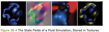
Our simulation represents data on a two-dimensional grid. The natural representation for this grid on the CPU is an array. The analog of an array on the GPU is a texture. Although textures are not as flexible as arrays, their flexibility is improving as graphics hardware evolves. Textures on current GPUs support all the basic operations necessary to implement a fluid simulation. Because textures usually have three or four color channels, they provide a natural data structure for vector data types with two to four components. Alternatively, multiple scalar fields can be stored in a single texture. The most basic operation is an array (or memory) read, which is accomplished by using a texture lookup. Thus, the GPU analog of an array offset is a texture coordinate. We need at least two textures to represent the state of the fluid: one for velocity and one for pressure. In order to visualize the flow, we maintain an additional texture that contains a quantity carried by the fluid. We can think of this as “ink.” Figure 38-4 shows examples of these textures, as well as an additional texture for vorticity, described in Section 38.5.1.
Loop Bodies = Fragment Programs
A CPU implementation of the simulation performs the steps in the algorithm by looping, using a pair of nested loops to iterate over each cell in the grid. At each cell, the same computation is performed. GPUs do not have the capability to perform this inner loop over each texel in a texture. However, the fragment pipeline is designed to perform identical computations at each fragment. To the programmer, it appears as if there is a processor for each fragment, and that all fragments are updated simultaneously. In the parlance of parallel programming, this model is known as single instruction, multiple data (SIMD) computation. Thus, the GPU analog of computation inside nested loops over an array is a fragment program applied in SIMD fashion to each fragment.
Feedback = Texture Update
In Section 38.2.4, we described how we use Jacobi iteration to solve Poisson equations. This type of iterative method uses the result of an iteration as input for the next iteration. This feedback is common in numerical methods. In a CPU implementation, one typically does not even consider feedback, because it is trivially implemented using variables and arrays that can be both read and written. On the GPU, though, the output of fragment processors is always written to the frame buffer. Think of the frame buffer as a two-dimensional array that cannot be directly read. There are two ways to get the contents of the frame buffer into a texture that can be read:
- Copy to texture (CTT) copies from the frame buffer to a texture.
- Render to texture (RTT) uses a texture as the frame buffer so the GPU can write directly to it.
CTT and RTT function equally well, but have a performance trade-off. For the sake of generality we do not assume the use of either and refer to the process of writing to a texture as a texture update.
Earlier we mentioned that, in practice, each of the five steps in the algorithm updates a temporary grid and then performs a swap. RTT requires the use of two textures to implement feedback, because the results of rendering to a texture while it is bound for reading are undefined. The swap in this case is merely a swap of texture IDs. The performance cost of RTT is therefore constant. CTT, on the other hand, requires only one texture. The frame buffer acts as a temporary grid, and a swap is performed by copying the data from the frame buffer to the texture. The performance cost of this copy is proportional to the texture size.
3.2 Slab Operations
We break down the steps of our simulation into what we call slab operations (slabop, for short). Each slabop consists of processing one or more (often all) fragments in the frame buffer—usually with a fragment program active—followed by a texture update. Fragment processing is driven by rendering geometric primitives. For this application, the geometry we render is simple: just quad and line primitives.
There are two types of fragments to process in any slab operation: interior fragments and boundary fragments. Our 2D grid reserves a single-cell perimeter to store and compute boundary conditions. Typically, a different computation is performed on the interior and at the boundaries. To update the interior fragments, we render a quadrilateral that covers all but a one-pixel border on the perimeter of the frame buffer. We render four line primitives to update the boundary cells. We apply separate fragment programs to interior and border fragments. See Figure 38-5.
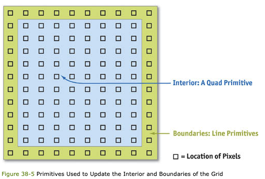
3.3 Implementation in Fragment Programs
Now that we know the steps of our algorithm, our data representation, and how to perform a slab operation, we can write the fragment programs that perform computations at each cell.
Advection
The fragment program implementation of advection shown in Listing 38-1 follows nearly exactly from Equation 13, repeated here:
Equation 13
There is one slight difference. Because texture coordinates are not in the same units as our simulation domain (the texture coordinates are in the range [0, N], where N is the grid resolution), we must scale the velocity into grid space. This is reflected in Cg code with the multiplication of the local velocity by the parameter , which represents the reciprocal of the grid scale . The texture wrap mode must be set to CLAMP_TO_EDGE so that back-tracing outside the range [0, N] will be clamped to the boundary texels. The boundary conditions described later correctly update these texels so that this situation operates correctly.
Example 38-1. Advection Fragment Program
1 | void advect(float2 coords : WPOS, // grid coordinates |
2 | out float4 xNew : COLOR, // advected qty |
3 | uniform float timestep, |
4 | uniform float rdx, // 1 / grid scale |
5 | uniform samplerRECT u, // input velocity |
6 | uniform samplerRECT x) // qty to advect |
7 | { |
8 | // follow the velocity field "back in time" |
9 | float2 pos = coords - timestep * rdx * f2texRECT(u, coords); |
10 | // interpolate and write to the output fragment |
11 | xNew = f4texRECTbilerp(x, pos); |
12 | } |
In this code, the parameter is the velocity field texture, and is the field that is to be advected. This could be the velocity or another quantity, such as dye concentration. The function f4texRECTbilerp() is a utility to perform bilinear interpolation of the four texels closest to the texture coordinates passed to it. Because current GPUs do not support automatic bilinear interpolation in floating-point textures, we must implement it with this type of code.
Viscous Diffusion
With the description of the Jacobi iteration technique given in Section 38.2.4, writing a Jacobi iteration fragment program is simple, as shown in Listing 38-2.
Example 38-2. The Jacobi Iteration Fragment Program Used to Solve Poisson Equations
1 | void jacobi(half2 coords : WPOS, // grid coordinates |
2 | out half4 xNew : COLOR, // result |
3 | uniform half alpha, |
4 | uniform half rBeta, // reciprocal beta |
5 | uniform samplerRECT x, // x vector (Ax = b) |
6 | uniform samplerRECT b) // b vector (Ax = b) |
7 | { |
8 | // left, right, bottom, and top x samples |
9 | half4 xL = h4texRECT(x, coords - half2(1, 0)); |
10 | half4 xR = h4texRECT(x, coords + half2(1, 0)); |
11 | half4 xB = h4texRECT(x, coords - half2(0, 1)); |
12 | half4 xT = h4texRECT(x, coords + half2(0, 1)); |
13 | |
14 | // b sample, from center |
15 | half4 bC = h4texRECT(b, coords); |
16 | // evaluate Jacobi iteration |
17 | xNew = (xL + xR + xB + xT + alpha * bC) * rBeta; |
18 | } |
Notice that the rBeta parameter is the reciprocal of b from Equation 16. To solve the diffusion equation, we set alpha to , rBeta to , and the and parameters to the velocity texture. We then run a number of iterations (usually 20 to 50, but more can be used to reduce the error).
Force Application
The simplest step in our algorithm is computing the acceleration caused by external forces. In the demonstration application found in the accompanying materials, you can apply an impulse to the fluid by clicking and dragging with the mouse. To implement this, we draw a spot into the velocity texture at the position of the click. The color of the spot encodes the direction and magnitude of the impulse: the red channel contains the magnitude in , and the green channel contains the magnitude in . The spot is actually a two-dimensional Gaussian “splat.”
We use a fragment program to check each fragment’s distance from the impulse position. Then we add the quantity to the color:
Here, is the force computed from the direction and length of the mouse drag, is the desired impulse radius, and and are the fragment position and impulse (click) position in window coordinates, respectively.
Projection
In the beginning of this section, we learned that the projection step is divided into two operations: solving the Poisson-pressure equation for , and subtracting the gradient of from the intermediate velocity field. This requires three fragment programs: the aforementioned Jacobi iteration program, a program to compute the divergence of the intermediate velocity field, and a program to subtract the gradient of from the intermediate velocity field.
The divergence program shown in Listing 38-3 takes the intermediate velocity field as parameter and one-half of the reciprocal of the grid scale as parameter halfr, and it computes the divergence according to the finite difference formula given in Table 38-1, on page 643.
The divergence is written to a temporary texture, which is then used as input to the parameter of the Jacobi iteration program. The parameter of the Jacobi program is set to the pressure texture, which is first cleared to all zero values (in other words, we are using zero as our initial guess for the pressure field). The alpha and rBeta parameters are set to and , respectively.
To achieve good convergence on the solution, we typically use 40 to 80 Jacobi iterations. Changing the number of Jacobi iterations will affect the accuracy of the simulation. It is not a good idea to go below 20 iterations, because the error is noticeable. Using more iterations results in more detailed vortices and more overall accuracy, but it requires more computation time. After the Jacobi iterations are finished, we bind the pressure field texture to the parameter in the following program, which computes the gradient of according to the definition in Table 38-1 and subtracts it from the intermediate velocity field texture in parameter . See Listing 38-4.
Example 38-3. The Divergence Fragment Program
1 | void divergence(half2 coords : WPOS, // grid coordinates |
2 | out half4 div : COLOR, // divergence |
3 | uniform half halfrdx, // 0.5 / gridscale |
4 | uniform samplerRECT w) // vector field |
5 | { |
6 | half4 wL = h4texRECT(w, coords - half2(1, 0)); |
7 | half4 wR = h4texRECT(w, coords + half2(1, 0)); |
8 | half4 wB = h4texRECT(w, coords - half2(0, 1)); |
9 | half4 wT = h4texRECT(w, coords + half2(0, 1)); |
10 | |
11 | div = halfrdx * ((wR.x - wL.x) + (wT.y - wB.y)); |
12 | } |
Example 38-4. The Gradient Subtraction Fragment Program
1 | void gradient(half2 coords : WPOS, // grid coordinates |
2 | out half4 uNew : COLOR, // new velocity |
3 | uniform half halfrdx, // 0.5 / gridscale |
4 | uniform samplerRECT p, // pressure |
5 | uniform samplerRECT w) // velocity |
6 | { |
7 | half pL = h1texRECT(p, coords - half2(1, 0)); |
8 | half pR = h1texRECT(p, coords + half2(1, 0)); |
9 | half pB = h1texRECT(p, coords - half2(0, 1)); |
10 | half pT = h1texRECT(p, coords + half2(0, 1)); |
11 | |
12 | uNew = h4texRECT(w, coords); |
13 | uNew.xy -= halfrdx * half2(pR - pL, pT - pB); |
14 | } |
Boundary Conditions
In Section 38.2.4, we determined that our “fluid in a box” requires no-slip (zero) velocity boundary conditions and pure Neumann pressure boundary conditions. In Section 38.3.2 we learned that we can implement boundary conditions by reserving the one-pixel perimeter of our grid for storing boundary values. We update these values by drawing line primitives over the border, using a fragment program that sets the values appropriately.
First we should look at how our grid discretization affects the computation of boundary conditions. The no-slip condition dictates that velocity equals zero on the boundaries, and the pure Neumann pressure condition requires the normal pressure derivative to be zero at the boundaries. The boundary is defined to lie on the edge between the boundary cell and its nearest interior cell, but grid values are defined at cell centers. Therefore, we must compute boundary values such that the average of the two cells adjacent to any edge satisfies the boundary condition.
For the velocity boundary on the left side, for example, we have:
Equation 17
where is the grid resolution. In order to satisfy this equation, we must set equal to . The pressure equation works out similarly. Using the forward difference approximation of the derivative, we get:
Equation 18
On solving this equation for , we see that we need to set each pressure boundary value to the value just inside the boundary.
We can use a simple fragment program for both the pressure and the velocity boundaries, as shown in Listing 38-5.
Example 38-5. The Boundary Condition Fragment Program
1 | void boundary(half2 coords : WPOS, // grid coordinates |
2 | half2 offset : TEX1, // boundary offset |
3 | out half4 bv : COLOR, // output value |
4 | uniform half scale, // scale parameter |
5 | uniform samplerRECT x) // state field |
6 | { |
7 | bv = scale * h4texRECT(x, coords + offset); |
8 | } |
Figure 38-6 demonstrates how this program works. The parameter represents the texture (velocity or pressure field) from which we read interior values. The offset parameter contains the correct offset to the interior cells adjacent to the current boundary. The coords parameter contains the position in texture coordinates of the fragment being processed, so adding offset to it addresses a neighboring texel. At each boundary, we set offset to adjust our texture coordinates to the texel just inside the boundary. For the left boundary, we set it to (1, 0), so that it addresses the texel just to the right; for the bottom boundary, we use (0, 1); and so on. The scale parameter can be used to scale the value we copy to the boundary. For velocity boundaries, scale is set to -1, and for pressure it is set to 1, so that we correctly implement Equations 17 and 18, respectively.
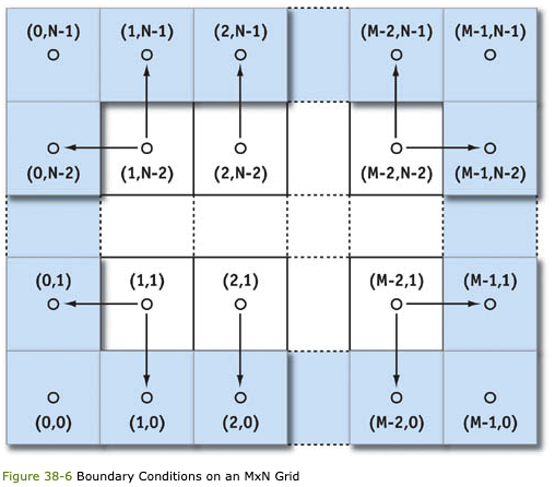
4 Applications
In this section we explore a variety of applications of the GPU simulation techniques discussed in this chapter.
4.1 Simulating Liquids and Gases
The most direct use of the simulation techniques is to simulate a continuous volume of a liquid or gas. As it stands, the simulation represents only the velocity of the fluid, which is not very interesting. It is more interesting if we put something else in the fluid. The demonstration application does this by maintaining an additional scalar field. This field represents the concentration of dye carried by the fluid. (Because it is an RGB texture, it is really three scalar fields: one for each of three dye colors.) Quantities like this are known as passive scalars because they are only carried along by the fluid; they do not affect how it flows.
If is the concentration of dye, then the evolution of the dye field is governed by the following equation:
To simulate how the dye is carried by the fluid, we apply the advection operator to the scalar field, just as we do for the velocity. If we also want to account for the diffusion of the dye in the fluid, we add a diffusion term:
where is the coefficient of the diffusion of dye in water (or whatever liquid we assume the fluid is). To implement dye diffusion, we use Jacobi iteration, just as we did for viscous diffusion of velocity. Note that the demonstration application does not actually perform diffusion of the dye, because numerical error in the advection term causes it to diffuse anyway. We added another term to . This term represents any sources of dye. The application implements this term by adding dye anywhere we click.
4.2 Buoyancy and Convection
Temperature is an important factor in the flow of many fluids. Convection currents are caused by the changes in density associated with temperature changes. These currents affect our weather, our oceans and lakes, and even our coffee. To simulate these effects, we need to add buoyancy to our simulation.
The simplest way to incorporate buoyancy is to add a new scalar field for temperature, , to the simulation. We can then insert an additional buoyancy operator that adds force where the local temperature is higher than a given ambient temperature, :
In this equation, is the vertical direction and s is a constant scale factor. This force can be implemented in a simple fragment program that evaluates the equation at each fragment, scales the result by the time step, and adds it to the current velocity.
Smoke and Clouds
We now have almost everything we need to simulate smoke. What we have presented so far is similar to the smoke simulation technique introduced by Fedkiw et al. 2001. In addition to calculating the velocity and pressure fields, a smoke simulation must maintain scalar fields for smoke density, , and temperature, . The smoke density is advected by the velocity field, just like the dye we described earlier. The buoyant force is modified to account for the gravitational pull on dense smoke:
where is a constant mass scale factor.
By adding a source of smoke density and temperature (possibly representing a smokestack or the tip of a cigarette) at a given location on the grid, we simulate smoke. The paper by Fedkiw et al. describes two other differences from our basic simulation. They use a staggered grid to improve accuracy, and they add a vorticity confinement force to increase the amount of swirling motion in the smoke. Both extensions are discussed in the next section.
As demonstrated in Harris et al. 2003, a more complex simulation can be used to simulate clouds on the GPU. A sequence of stills from a 2D GPU cloud simulation is shown in Figure 38-7. The cloud simulator combines fluid simulation with a thermodynamic simulation (including buoyancy), as well as a simulation of water condensation and evaporation. A 128x128 cloud simulation runs at over 80 iterations per second on an NVIDIA GeForce FX 5950 Ultra GPU.
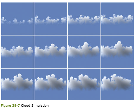
5 Extensions
The fluid simulation presented in this chapter is a building block that can serve as the basis for more complex simulations. There are many ways to extend this basic simulation. To get you started, we describe some useful extensions.
5.1 Vorticity Confinement
The motion of smoke, air and other low-viscosity fluids typically contains rotational flows at a variety of scales. This rotational flow is vorticity. As Fedkiw et al. explained, numerical dissipation caused by simulation on a coarse grid damps out these interesting features (Fedkiw et al. 2001). Therefore, they used vorticity confinement to restore these fine-scale motions. Vorticity confinement works by first computing the vorticity, . From the vorticity we compute a normalized vorticity vector field:
here, $ \eta = \nabla |\omega|$. The vectors in this vector field point from areas of lower vorticity to areas of higher vorticity. From these vectors we compute a force that can be used to restore an approximation of the dissipated vorticity:
.
Here is a user-controlled scale parameter. The “curl” operator, , can be derived using the definitions of the gradient and the cross-product operator. The accompanying source code implements vorticity confinement.
5.2 Three Dimensions
All the simulations presented in this chapter are two-dimensional. There is nothing preventing us from extending them to 3D. The equations remain essentially the same, but we must extend them to incorporate a 3D velocity, . The fragment programs must be rewritten to account for this; samples from four neighbors in two dimensions become samples from six neighbors in three dimensions.
The biggest change is in how the vector and scalar fields are represented. One option is to use 3D textures. This is a problem on hardware that does not support 3D floating-point textures. In this situation, we can tile the slabs of a 3D texture in a grid stored in a 2D texture (for example, a 32x32x32 grid would tile onto a 256x128 2D texture, with eight tiles in one dimension and four in the other). This technique, called flat 3D textures, is presented in detail in Harris et al. 2003.
5.3 Staggered Grid
In our simulation we represent velocity, pressure, and any other quantities at cell centers. This is just one way to discretize the continuous domain on which we represent our fluid. This approach is known as a collocated, or cell-centered, discretization. Another way is to use a staggered grid. In a staggered grid, we represent scalar quantities (such as pressure) at cell centers and vector quantities (such as velocity) at the boundaries between cells. Specifically, on a two-dimensional grid, we represent the horizontal velocity, u, at the right edge of each cell and the vertical velocity, v, at the top edge of each cell. The staggered grid discretization increases the accuracy of many calculations. It can also reduce numerical oscillations that may arise when forces such as buoyancy are applied on a cell-centered grid. Details of the implementation of fluid simulation on a staggered grid can be found in Griebel et al. 1998.
5.4 Arbitrary Boundaries
So far we have assumed that our fluid exists in a rectangular box with flat, solid sides. If boundaries of arbitrary shape and location are important, you need to extend the simulation.
Incorporating arbitrary boundaries requires applying the boundary conditions (discussed in Section 38.3.3) at arbitrary locations. This means that at each cell, we must determine in which direction the boundaries lie in order to compute the correct boundary values. This simulation requires more decisions to be made at each cell, leading to a slower and more complicated simulation. However, many interesting effects can be created this way, such as smoke flowing around obstacles. Moving boundaries can even be incorporated, as in Fedkiw et al. 2001. We refer you to that paper as well as Griebel et al. 1998 for implementation details.
5.5 Free Surface Flow
Another assumption we made is that our fluid is continuous—the only boundaries we represent are the solid boundaries of the box. So we cannot simulate things like the ocean surface, where there is an interface between the water and air. This type of interface is called a free surface. Extending our simulation to incorporate a free surface requires tracking the location of the surface as it moves through cells. Methods for implementing free surface flow can be found in Griebel et al. 1998.
6 Conclusion
The power and programmability now available in GPUs enables fast simulation of a wide variety of phenomena. Underlying many of these phenomena is the dynamics of fluid motion.
After reading this chapter, you should have a fundamental understanding of the mathematics and technology you need to implement basic fluid simulations on the GPU. From these initial ideas you can experiment with your own simulation concepts and incorporate fluid simulation into graphics applications. We hope these techniques become powerful new tools in your repertoire.
前向后项差分和显式隐式欧拉法
主要介绍前向后向差分,显式隐式欧拉法及其稳定性分析。
前向差分对应显式方法,后向差分对应隐式方法。显式欧拉法是比较流行的显式方法,隐式欧拉法是比较流行的隐式方法。
显式欧拉法条件稳定,对积分步长有要求,隐式欧拉法无条件稳定,对积分步长无要求(理论上如此,但实际使用中对积分步长仍然有要求,只是比显式欧拉宽松)。
前向差分与后向差分
设一元函数函数离散化为一系列的点,其中,, , 为步长。
前向差分(Forward Difference)
前向差分的定义:.
之所以称之为前向差分,是因为当前时刻的差分,是下一时刻位置(时间向前前进一步)与当前时刻位置之差。高阶前向差分
根据上式递归可得阶前向差分公式为:.
例如,二阶前向差分公式为:
后向差分(Backward Difference)
后向差分定义:.
由定义可以看出,当前时刻的差分,是当前时刻的位置与前一时刻的位置之差。高阶后向差分
同上,k阶后向差分公式为:.
因此,二阶后向差分公式为:.
差商和导数
差商就是差分除以步长,即 .
在数值计算中,需要以差商代替导数,即
如果使用前向差分,则为显式方法,例如
如果使用后向差分,则为隐式方法,例如
显式欧拉和隐式欧拉
设有一阶常微分方程.很多时候我们无法求出函数yy的解析解,只能通过数值方法逼近,即,将时间离散为一系列的点其中, 我们要做的就是求函数y在这些离散的时间点上的值.
显式欧拉(Explicit Euler)
显式欧拉公式:
之所以称之为显式,是因为下一时刻的值,可根据当前时刻的值及其导数 显式地给出。
另一种角度看上面的公式:从当前时刻出发,根据当前时刻的函数值及其导数,可得到下一时刻的值。因此显式欧拉法又称为前向欧拉(Forward Euler)
再从另一个角度看,我们把上面的公式做一下变形可得. 即,显示欧拉就是用前向差商代替导数。
隐式欧拉(Implicit Euler)
隐式欧拉公式:
之所以称之为隐式,是因为上式是一个隐式方程。
另一种角度看上面的公式:将上式做一下变形可得:.从当前时刻出发,根据当前时刻的函数值及其导数,可得到前一时刻函数的值。因此隐式欧拉法又称为后向欧拉(Backward Euler)
再从另一个角度看,我们把上面的公式做一下变形可得. 即,显示欧拉就是用前向差商代替导数。
例证欧拉法的稳定性
设有一阶常微分方程. 我们知道,这个常微分方程的解析解为. 当. 那么分别用显式、隐式欧拉法会得到什么呢?
-
显式欧拉法条件稳定(Conditionally Stable)
根据显式欧拉法公式
为了保证上式收敛,需要保证, 得,, 即,条件稳定. -
隐式欧拉法无条件稳定(Unconditionally Stable)
根据隐式欧拉公式,.
则, .
又,则恒大于1。即不管时间步长为多大,隐式欧拉始终稳定,即无条件稳定.
实际应用中,隐式欧拉需要求解隐式方程,通常也是使用逼近的方法(例如,Newton-Raphson)求解,因此实际的隐式欧拉方法并不是无条件稳定的。