Linear Algebra and Matrix Analysis(线性代数和矩阵分析)

linear-algebra

Solving Linear Equations

Rules:

1. $(AB)^{-1} = B^{-1}A^{-1}$
2. $A^{-1}A = I = AA^{-1}$
3. $(AB)\mathbf x = A(B\mathbf x)$
4. $A = LU = (\text{lower triangular}) (\text{upper triangular}) = LDU$

A = L U is “unsymmetric” because U has the pivots on its diagonal where L has l’s. This is easy to change. Divide U by a diagonal matrix D that contains the pivots. That leaves a new triangular matrix with l’s on the diagonal:
Split U into $\begin{bmatrix}d_1 & & & \\ & d_2 & & \\ & & \ddots & \\ & & & d_n \end{bmatrix}\begin{bmatrix} 1 & u_{12}/d_1 & u_{13}/d_1 & . \\ & 1 & u_{23}/d_2 & . \\ & & \ddots & \vdots \\ & & & 1\end{bmatrix}$

5. $(AB)^T = B^TA^T$

Vector Spaces and Subspaces

1. A real vector space is a set of “vectors” together with rules for vector addition and for multiplication by real numbers.
2. A subspace of a vector space is a set of vectors (including 0) that satisfies two requirements: If $\mathbf v$ and $\mathbf w$ are vectors in the subspace and c is any scalar, then

1. $\mathbf v$ + $\mathbf w$ is in the subspace.
2. $c\mathbf v$ is in the subspace.

3. A subspace containing v and w must contain all linear combinations $c\mathbf v$ + $d\mathbf w$.
4. The column space consists of all linear combinations of the columns .The combinations are all possible vectors $A\mathbf x$. They fill the column space $\mathbf C(A)$.
   For example $A\mathbf x$ is $\begin{bmatrix} 1 & 0 \\ 4 & 3 \\ 2 & 3\end{bmatrix}\begin{bmatrix}x_1 \\ x_2\end{bmatrix}$ which is $x_1\begin{bmatrix} 1\\ 4\\ 2\end{bmatrix} + x_2\begin{bmatrix} 0 \\3 \\ 3\end{bmatrix}$

This column space is crucial., To solve $A\mathbf x = \mathbf b$ is to express $\mathbf b$ as a combination ofthe columns.

The system $A\mathbf x = \mathbf b$ is solvable if and only if $\mathbf b$ is in the column space of A.

5. The nullspace $N(A)$ in $R^n$ contains all solutions $\mathbf x$ to $A\mathbf x = 0$. This include $\mathbf x = 0$
6. Elimination (from $A$ to $U$ to $R$) does not change the nullspace: $N(A) = N(U)= N(R)$.
7. Suppose $A\mathbf x = 0$ has more unknowns than equations (n > m, more columns than rows). There must be at least one free column. Then Ax = 0 has nonzero solutions.

A short wide matrix $(n > m)$ always has nonzero vectors in its nullspace. There must be at least $n - m$ free variables, since the number of pivots cannot exceed m. (The matrix only has m rows, and a row never has two pivots.) Of course a row might have no pivot­ which means an extra free variable. But here is the point: When there is a free variable, it can be set to 1. Then the equation $A\mathbf x = 0$ has at least a line of nonzero solutions.

8. The nullspace is a subspace. Its “dimension” is the number of free variables. This central idea-the dimension of a subspace
9. The rank of $A$ is the number of pivots. This number is $r$. Every ''free column" is a combination of earlier pivot columns. It is the special solutions $\mathbf s$ that tell us those combinations.

$\text{Number of pivots} = \text{number of nonzero rows in R}= \text{rank } \mathbf r$. There are $n - r$ free columns.

10. The column space of a rank one matrix is “one-dimensional”, have the special rank one form $A = \mathbf {uv}^T$, which is form the rank one matrix, $A = \text{column times row} = \mathbf {uv}^T$ , $\mathbf u, \mathbf v$ are basis vector.
11. Complete solution to $A\mathbf x = b$ is that
    $\mathbf x = \text{(one particular solution } \mathbf x_p \text{) + (any } \mathbf x_n \text{ in the nullspace)}$

The particular solutioni solves $A\mathbf x_p = b$
The $n - r$ special solutions solve $A\mathbf x_n = 0$
it means $A\mathbf x_p + A\mathbf x_n = A(\mathbf x_p + \mathbf x_n) = b + 0 = b$

Suppose $A$ is a square invertible matrix, $m = n = r$. The particular solution is the one and only solution $\mathbf x_p = A^{-1}b$. There are no special solutions or free variables.
$R = I$ has no zero rows. The only vectorin the nullspace is $\mathbf x_n = 0$. The complete solution is $\mathbf x =\mathbf x_p + \mathbf x_n = A^{-1}b + 0$.

12. Every matrix $A$ with full column rank (r = n) has all these properties:

1. All columns of $A$ are pivot columns.
2. There are no free variables or special solutions.
3. The nullspace $N(A)$ contains only the zero vector $\mathbf x = 0$.
4. If $A\mathbf x = b$ has a solution (it might not) then it has only one solution.

13. Every matrix $A$ with full row rank (r = m) has all these properties:

1. All rows have pivots, and R has nozero rows.
2. $A\mathbf x = b$ has a solution for every right side b.
3. The column space is the whole space $R^m$
4. There are $n - r = n - m$ special solutions in the nullspace of $A$.

In this case with $m$ pivots, the rows are “linearly independent”. So the columns of $A^T$ are linearly independent. The nullspace of $A^T$ is the zero vector.

14. The columns of $A$ are linearly independent when the only solution to $A\mathbf x = 0$ is $x = 0$. No other combination $A\mathbf x$ of the columns gives the zero vector.
15. The sequence of vectors $v_1, \cdots , v_n$ is linearly independent if the only combination that gives the zero vector is $0v_1 + 0v_2 + \cdots + 0v_n$. that’s $x_1v_1 + x_2v_2 + \cdots + x_nv_n = 0$ only happens when all $x$'s are zero.
16. The row space of $A$ is $C(A^T)$, it’s the column space of $A^T$
17. The vectors $v_1, \cdots , v_n$ are a basis for $R^n$ exactly when they are the columns of an $n \times n$ invertible matrix. Thus $R^n$ has infinitely many different bases.

The pivot columns of $A$ are a basis for its column space. The pivot rows of $A$ are a basis for its row space. So are the pivot rows of its echelon form $R$.

18. If $v_1,\cdots, v_m$ and $w_1, \cdots, w_n$ are both bases for the same vector space, then $m = n$. The dimension of a space is the number of vectors in every basis.

For example
for the matrix $A = \begin{bmatrix} 1 & 2 & 3 \\ 2 & 2 & 8\end{bmatrix}$ the column space $C(A)$ and the row space $C(A^T)$ has a dimension 2, not 3
for the matrix $B = \begin{bmatrix} 1 & 2\\ 2 & 2 \\ 3& 8 \end{bmatrix}$ the column space $C(B)$ and the row space $C(B^T)$ has a dimension 2, not 3

19. Four Fundamental Subspaces of matrix $A_{m \times n}$

1. The row space is $C(A^T)$, a subspace of $R^n$.
2. The column space is $C(A)$, a subspace of $R^m$.
3. The nullspace is $N(A)$, a subspace of $R^n$
4. The left nullspace is $N(A^T)$, a subspae of $R^m$.
   For the left nullspace we solve $A^T\mathbf y = 0$(the system is $n\times m$. it is the nullspace of $A^T$).
   The vectors $\mathbf y$ go on the left side of $A$ when the equation is written $y^TA = 0^T$ .

The row space and column space have the same dimension $r = \text{Rank}(A)$.
$N(A)$ and $N(A^T)$ have dimensions $n - r$ and $m - r$, to make up the full $n$ and $m$.

In $R^n$ the row space and nullspace have dimensions $r$ and $n-r$
In $R^m$ the column space and left nullspace have dimensions $r$ and $m - r$

20. A matrix multiplies a vector: $A$ times $\mathbf x$.

• At the first level this is only numbers.
• At the second level $A\mathbf x$ is a combination of column vectors.
• The third level shows subspaces. The matrix $A_{m\times n}$'s big picture as follow
  

1. The row space is perpendicular to the nullspace.
   Every row of $A$ is perpendicular to every solution of $A\mathbf x = 0$.
2. The column space is perpendicular to the nullspace of $A^T$
   When $b$ is outside the column space—when we want to solve $A\mathbf x = b$ and can’t do it—then this nullspace of $A^T$ comes into its own. It contains the error $e = b - A\mathbf x$ in the “least-squares” solution.

21. Every rank one matrix is one column times one row $A= \mathbf u\mathbf v^T$.
    Rank Two Matrices = Rank One plus Rank One

For example as follow
$A = \begin{bmatrix} 1 & 0 & 3 \\ 1&1&7 \\ 4&2&20\end{bmatrix} = \begin{bmatrix}1&0&0\\1&1&0\\4&2&1\end{bmatrix}\begin{bmatrix}1&0&3\\0&1&4\\0&0&0\end{bmatrix} = CR$
The row space of $R$ clearly has two basis vectors $v_1^T = \text{[1 0 3]}$ and $v_2^T = \text{[0 1 4]}$. and the column space of $C$ clearly has tow basic vectors $u_1 = \text{(1,1,4)}, u_2 = \text{(0,1,2)}$, Then
$A = \begin{bmatrix}u_1&u_2&u_3\end{bmatrix} \begin{bmatrix}v_1^T\\v_2^T\\\text{zero row}\end{bmatrix} = u_1v_1^T + u_2v_2^T = (\text{rank 1}) + (\text{rank 1})$

Orthogonality

Orthogonality of the Four Subspaces

1. Orthogonality of the Four Subspaces

1. Orthogonal vectors have $\mathbf v^T\mathbf w=0$.Then $||\mathbf v^2||+||\mathbf w^2||= ||\mathbf v + \mathbf w||^2 = ||\mathbf v - \mathbf w||^2$
2. Subspaces $V$ and $W$ are orthogonal when $\mathbf v^T\mathbf w = 0$ for every $\mathbf v$ in $V$ and every $\mathbf w$ in $W$.
3. The row space of $A$ is orthogonal to the nullspace. The column space is orthogonal to $N(A^T)$.
4. Row space and nullspace are orthogonal complements: Every $x$ in $R^n$ splits into $X_{row} + X_{null}$·

2. Every vector $\mathbf x$ in the nullspace is perpendicular to every row of $A$, because $A\mathbf x = 0$.
   The nullspace $N(A)$ and the row space $C(A^T)$ are orthogonal subspaces of $R^n$ .

Proof as follow
$A\mathbf x = \begin{bmatrix}row\space 1 \\ \vdots \\ row\space m\end{bmatrix}\begin{bmatrix}\mathbf x\end{bmatrix} = \begin{bmatrix}0\\ \vdots \\0\end{bmatrix}$. It’s cleary that $\text{(row m)} \cdot x $ is zero.
Or the seccond way to proof that orthogonality for readers who like matrix shorthand. The vectors in the row space are combinations $A^Ty$ of the rows.
Take the dot product of $A^Ty$ with any $x$ in the nullspace. These vectors are perpendicular:
$\mathbf x^T(A^Ty) = (A\mathbf x)^Ty = 0^Ty = 0$

3. Every vector $y$ in the nullspace of $A^T$ is perpendicular to every column of A.
   The left nullspace $N(A^T)$ and the column space $C(A)$ are orthogonal in $R^m$.

For a visual proof, look at $A^Ty = 0$. Each column of $A$ multiplies $y$ to give 0:
$C(A) \perp N(A^T)$ which is $A^Ty = \begin{bmatrix}\text{(column 1)}^T \\ \cdots \\ \text{(column n)}^T\end{bmatrix} \begin{bmatrix}y\end{bmatrix} = \begin{bmatrix}0 \\ .\\0\end{bmatrix}$
The dot product of $y$ with every column of $A$ is zero. Then $y$ in the left nullspace is perpendicular to each column of $A$—and to the whole column space.

4. The orthogonal complement of a subspace $V$ contains every vector that is perpendicular to $V$. This orthogonal subspace is denoted by $V^{\perp}$(pronounced"$V$ perp").
   By this definition, the nullspace is the orthogonal complement of the row space.

Every $x$ that is perpendicular to the rows satisfies $A\mathbf x = 0$, and lies in the nullspace.

The reverse is also true. If $v$ is orthogonal to the nullspace, it must be in the row space.
Otherwise we could add this $v$ as an extra row of the matrix, without changing its nullspace. The row space would grow, which breaks the law $r + (n - r) = n$. We conclude that the nullspace complement $N(A)^{\perp}$ is exactly the row space $C(A^T)$.

In the same way, the left nullspace and column space are orthogonal in $R^m$, and they are orthogonal complements. Their dimensions $r$ and $m - r$ add to the full dimension $m$.

1. $N(A)$ is the orthogonal complement ofthe row space $C(A^T)$ (in $R^n$).
2. $N(A^T)$ is the orthogonal complement of the column space $C(A)$ (in $R^m$ ).

The point of **“complements” **is that every $\mathbf x$ can be split into a row space component $\mathbf r$ and a nullspace component $\mathbf x_n$ . When A multiplies $\mathbf x = \mathbf x_r + \mathbf x_n$ , Figure below shows what happens to $A\mathbf x= A\mathbf {x_r} + A\mathbf {x_n}$ :

The nullspace component goes to zero: $A\mathbf {x_n} =0$.
The row space component goes to the column space: $A\mathbf {x_r} = A\mathbf x$.

Every vector goes to the column space!
Multiplying by $A$ cannot do anything else. More than that: Every vector $b$ in the column space comes from one and only one vector $\mathbf x_r$ in the row space.

Proof: If $A\mathbf {x_r} = A\mathbf x_r'$, the difference $\mathbf x_r - \mathbf x_r'$ is in the nullspace. It is also in the row space, where $\mathbf x_r$ and $\mathbf x_r'$ came from. This difference must be the zero vector, because the nullspace and row space are perpendicular. Therefore $\mathbf x_r = \mathbf x_r'$

5. repeat one clear fact. A row of $A$ can’t be in the nullspace of A (except for a zero row). The only vector in two orthogonal subspaces is the zero vector.

Projections

1. The projection of a vector $b$ onto the line through $a$ is the closest point $p=a\frac{a^Tb}{a^Ta}$.
   The projection matrix $P = \frac{aa^T}{a^Ta}$

$p = \lambda a = a \lambda = a\frac{a^Tb}{a^Ta} = \frac{aa^T}{a^Ta}b= Pb$, then the P is the projection matrix that handle the transform, p is the projection result vector.

The error $e = b-p$ is perpendicular to $a$ : Right triangle $b,p,e$ has rulle $||p|| + ||e|| = ||b||$.
2. The projection of $b$ onto a subspace $S$ is the closest vector $p$ in $S$; $b - p$ is orthogonal to $S$.

Assume n linearly independent. vectors $a_1, \cdots , a_n$ in $R^m$.
Find the combination $p = \hat x_1 a_1 + \cdots + \hat x_n a_n$ closest to $a$ given vector $b$.

We compute projections onto $n-dimensional subspaces in 3 steps as before:

1. find the vector $\mathbf x$
2. find the projection $p = A\mathbf x$
3. find the projection matrix $P$

The key is $b$ to the nearest point $A\hat{\mathbf x}$ in the subspace. This error vector $b - A\hat{\mathbf x}$ is perpendicular to the subspace. The error $b - A\hat{\mathbf x}$ makes a right angle with all the vectors $a_1,\cdots,a_n$ in the base. The $n$ right angles give the $n$ equations for $\hat{\mathbf x}$:
$\begin{bmatrix}-a_1^T-\\ \vdots \\ -a_n^T-\end{bmatrix}\begin{bmatrix}b - A\hat{\mathbf x}\end{bmatrix} = \begin{bmatrix}0\end{bmatrix}$
The matrix with those rows $a_i^T$ is $A^T$. The $n$ equations are exactly $A^T(b - A\hat{\mathbf x}) = 0$.
Rewrite $A^T(b - A\hat{\mathbf x}) = 0$ in tis famous form $A^TA\hat{\mathbf x} = A^Tb$

The combination $p=\hat x_1a_1 + \cdots + \hat x_n a_n =Ax$ that is closest to $b$ comes from $\hat x$:
Find $\hat x(n\times 1) \to A^T(b - A\hat{\mathbf x}) = 0$ Or $A^TA\hat{\mathbf x} = A^Tb$
This symmetric matrix $A^TA$ is n by n. It is invertible if the a’s are independent.
The solution is $\hat x = (A^TA)^{-1}A^Tb$. The projection of $b$ onto the subspace is $p$.
Find $p(m\times 1) \to p = A\hat x = (A^TA)^{-1}A^Tb$
The next formula picks out the projection matrix that is multiplying $b$ in above
Find $P(m\times m) \to P = A(A^TA)^{-1}A^T$

Compare with projection onto a line, when $A$ has only one column : $A^TA$ is $a^Ta$.
For $n = 1\to \hat x = \frac{a^Tb}{a^Ta}, \hspace{1em} p = a\frac{a^Tb}{a^Ta}, \hspace{1em} P = \frac{aa^T}{a^Ta}$

The key step was $A^T (b - A\hat x) = 0$. We can expressed it by geometry. Linear algebra gives this “normal equation” too, in a very quick and beautiful way :

1. Our subspace is the column space of $A$.
2. The error vector $b-A\hat x$ is perpendicular to that column space.
3. Therefore $b-A\hat x$ is in the nullspace of $A^T$, that means $A^T(b - A\hat x) = 0$

The left nullspace is important in projections. That nullspace of $A^T$ contains the error vector $e = b- A\hat x$. The vector $b$ is being split into the projection $p$ and the error $e = b - p$. Projection produces a right triangle with sides $p, e, b$.

3. $A^TA$ is invertible if and only if $A$ has linearly independent columns.

Least Squares Approximations

1. When $Ax=b$ has no solution, multiply by $A^T$ and solve $A^TAx=A^Tb$.

It often happens that $Ax = b$ has no solution. The usual reason is: too many equations.
The matrix $A$ has more rows than columns. There are more equations than unknowns ($m>n$). Then columns span a small part of m-dimensional space. Unless all measurements are perfect, $b$ is outside that column space of $A$. Elimination reaches an impossible equation and stops. But we can’t stop just because measurements include noise!
WIth the projection, we can reduce the dimension difference.

So SolvingI $A^TAx=A^Tb$ gives the projection $p=A\hat x$ of $b$ onto the column space of $A$.

2. When $Ax=b$ has no solution, xis the “least -squares solution”: $||b - A\hat x||^2 = minimum$.

Setting partial derivatives of $E = ||Ax - b||^2$ to zero ($\frac{\partial E}{\partial x_i} = 0$)also produces $A^TAx =A^Tb$.

3. To fit points $(t_1,b_1),\cdots,(t_m,b_m)$by a straightline ,$A$ has columns $(1,\cdots,1)$ and $(t_1,\cdots,t_m)$.

$Ax = b $ is $\begin{matrix} C + Dt_1 = b_1\\ C + Dt_2 = b_2 \\ \vdots\\ C + Dt_m = b_m\end{matrix}$ with $A = \begin{bmatrix}1 & t_1 \\ 1 & t_2 \\ \vdots & \vdots \\ 1 & t_m\end{bmatrix}$.
The column space is so thin that almost certainly $b$ is outside of it. When $b$ happens to lie in the column space, the points happen to lie on a line. In that case $b = p$. Then $Ax = b$ is solvable and the errors are $e = (0,\cdots, 0)$.

Turn the fitting points by a straight line to least squares and Solve $A^TA\hat x=A^Tb$ for $\hat x=(C,D)$. The errors are $e_i=b_i-C-Dt_i$

$A^TA = \begin{bmatrix}1 & \cdots & 1\\ t_1 & \cdots & t_m\end{bmatrix}\begin{bmatrix}1 & t_1 \\ \vdots & \vdots \\ 1 & t_m\end{bmatrix} = \begin{bmatrix}m & \sum t_i \\ \sum t_i & \sum t_i^2\end{bmatrix}$
$A^Tb = \begin{bmatrix}1 & \cdots & 1\\ t_1 & \cdots & t_m\end{bmatrix}\begin{bmatrix}b_1 \\ \vdots \\b_m\end{bmatrix} = \begin{bmatrix}\sum b_i & \sum t_ib_i\end{bmatrix}$
$A^TA\hat x=A^Tb \to \begin{bmatrix}m & \sum t_i \\ \sum t_i & \sum t_i^2\end{bmatrix}\begin{bmatrix}C \\ D\end{bmatrix} = \begin{bmatrix}\sum b_i \\ \sum t_ib_i\end{bmatrix}$

The best $\hat x = (C, D)$ is $(A^TA)^{-1}A^Tb$.

Orthonormal Bases and Gram-Schmidt

1. The columns $q_1,\cdots,q_n$ are orthonormal if $q_i^Tq_j = \begin{cases}0 & for\space i \ne j \\ 1 & for\space i = j\end{cases}$. Then $Q^TQ = 1$

If $Q$ is also square then $Q^T = Q^{-1}$
The least squares solution to $Q\mathbf x = b$ is $\hat{\mathbf x} = Q^Tb$. Projection of $b$ is $p = QQ^Tb = Pb$

2. With three independent vectors $a, b, c$ to construct three orthogonal vectors $A, B, C$.
   let $A = a$
   then $B = b - \frac{A^Tb}{A^TA}A$
   then $C = c - \frac{A^Tc}{A^TA}A - \frac{B^Tc}{B^TB}B$

The Factorization $A = QR$ with $q_1 = \frac{A}{||A||}, q_2 = \frac{B}{||B||}, q_3 = \frac{C}{||C||}$
$\begin{bmatrix}a & b & c\end{bmatrix} = \begin{bmatrix}q_1 & q_2 & q_3\end{bmatrix}\begin{bmatrix}q_1^Ta & q_1^Tb & q_1^Tc \\ & q_2^Tb & q_2^Tc\\ & & q_3^Tc\end{bmatrix}$, which also is $A = QR$
Clearly, $R = Q^TA$

3. With $A = QR \to A^TA = (QR)^TQR = R^TQ^TQR = R^TR$
   So The least squares equation as follow
   $A^TA\hat x = A^Tb \to R^TR\hat x = R^TQ^Tb \to R\hat x = Q^Tb$
   $\hat x = R^{-1}Q^Tb$

Determinants

1. The determinant of an n by n matrix can be found in three ways:

1. Pivot formula.

Multiply the $n$ pivots (times 1 or -1)

2. “Big” formula.

Add up $n!$ terms (times 1 or -1)

3. Cofactor formula.

Combine $n$ smaller determinants (times 1 or -1)

2. The properties of the determinant

1. The determinant of the n by n identity matrix is 1.
2. The determinant changes sign when two rows are exchanged (sign reversal).
3. The determinant is a linear function of each row separately(all other rows stay fixed)

If the first row is multiplied by $t$, the determinant is multiplied by $t$. If first rows are added, determinants are added. This rule only applies when the other rows do not change! Notice how e and d stay the same:
multiply row 1 by any number $t$, det is multiplied by $t\begin{bmatrix}ta & tb \\ c& d\end{bmatrix} = t\begin{bmatrix}a & b \\ c & d\end{bmatrix}$
add row 1 of $A$ to row 1 of $A'$, then determinants add $\begin{bmatrix}a + a' & b + b' \\ c& d\end{bmatrix} = \begin{bmatrix}a & b \\ c & d\end{bmatrix} + \begin{bmatrix}a' & b' \\ c & d\end{bmatrix}$

4. If two rows of $A$ are equal, then $det\space A = 0$.
5. Subtracting a multiple of one row from another row leaves det A unchanged.

The determinant is not changed by the usual elimination steps from $A$ to $U$.
Thus $det\space A = det\space U$. If we can find determinants of triangular matrices $U$, we can find determinants of all matrices $A$. Every row exchange reverses the sign, so always $det\space A= \pm det\space U$.

6. A matrix with a row of zeros has $det\space A = 0$.
7. If $A$ is triangular then $det\space A = a_{11}a_{22}\cdots a_{nn} = \text{product ofdiagonal entries}$.
8. If $A$ is singular then $det\space A=0$. If $A$ is invertible then $det\space A\ne 0$.
9. $det\space A= \pm det\space U = \pm(\text{product of the pivots})$
10. the determinant of $AB$ is $det\space A$ times $det\space B$, that $det(AB) = det(A) det(B) \text{ OR } |AB| = |A| |B|$

$(det\space A)(det \space A^{-1}) = det\space I = 1$

11. the transpose $A^T$ has the same determinant as $A$, that’s $det\space A= det \space A^T$

3. The Pivot Formula

When elimination leads to $A = LU$, the pivots $d_1 , \cdots , d_n$ are on the diagonal of the upper triangular $U$. If no row exchanges are involved, multiply those pivots to find the determinant:
$det\space A = (det\space L)(det\space U) = (1)(d_1d_2\cdots d_n)$
$(det\space P)(det\space A) = (det\space L)(det\space U) \to det\space A = \pm(d_1d_2\cdots d_n).$
Each pivot is a ratio of determinants, the $k_{th}$ pivot is $d_k = \frac{d_1d_2\cdots d_k}{d_1d_2\cdots d_{k-1}} = \frac{det\space A_k}{det\space A_{k-1}}$

4. The Big Formula for Determinants

The formula has $n!$ terms. Its size grows fast because $n! = 1, 2, 6, 24, 120, \cdots $
The determinant of $A$ is the sum of these n! simple determinants times 1 or -1.
The simple determinants $a_{1\alpha}a_{2\beta}\cdots a_{n\omega}$ choose one entry from every row and column.

$det\space A\\ = \text{sum over all n! column permutations} P = (\alpha, \beta, \cdots, \omega)\\ = \sum(det\space P)a_{1\alpha}a_{2\beta}\cdots a_{n\omega} \\ = Big Formula$

5. Determinant by Cofactors

The determinant is the dot product of any row $i$ of $A$ with its cofactors using other rows:
Cofactors Formula $det \space A = a_{i1}C_{i1} + a_{i2}C_{i2} + \cdots + a_{in}C_{in}$
Each cofactor $C_{ij}$ (order $n - l$, without row $i$ and column $j$) includes its correct sign:
Cofactor $C_{ij} = (-1)^{i+j}det\space M_{ij}$
the submatrix $M_{ij}$ throws out row $i$ and column $j$.

Cramer’s Rule, Inverses, and Volumes

1. The Cramer’s Rule solves $Ax = b$

A neat idea gives the first component $x_1$ . Replacing the first column of $I$ by $x$ gives a matrix with determinant $x_1$ . When you multiply it by A, thefirst column becomes $Ax$ which is $b$. The other columns of $B_1$ are copied from $A$:
Key Idea $\begin{bmatrix}A\end{bmatrix} \begin{bmatrix}x_1 & 0 & 0 \\ x_2 & 1 & 0 \\ x_3 & 0 &1\end{bmatrix} = \begin{bmatrix}b_1 & a_{12} & a_{13} \\ b_2 & a_{22} & a_{23} \\ b_3 & a_{32} & a_{33}\end{bmatrix} = B_1$
With Product Rule $(det \space A)(det \begin{bmatrix}x_1 & 0 & 0 \\ x_2 & 1 & 0 \\ x_3 & 0 &1\end{bmatrix} ) = det\space B_1 \to (det \space A)(x_1) = det\space B_1 \to x_1 = \frac{det \space B_1}{det \space A}$
Wihe same procedure $x_2 = \frac{det \space B_2}{det \space A}, x_3 = \frac{det \space B_3}{det \space A}$

If $det\space A$ is not zero, $Ax = b$ is solved by determinants: $x_1 = \frac{det \space B_1}{det \space A}, x_2 = \frac{det \space B_2}{det \space A}, x_n = \frac{det \space B_n}{det \space A}$

The matrix $B_j$ has the $j_{th}$ column of $A$ replaced by the vector $b$.

2. $A^{-1}$ involves the cofactors. When the right side is a column of the identity matrix $I$, as in $AA^{-1} = I$,
   the determinant of each $B_j$ in Cramer’s Rule is a cofactor of $A$.

The $i,j$ entry of $A^{-1}$ is the cofactor $C_{ji} (notC_{ij})$ divided by $det\space A$.
$\displaystyle \text{Formula For } A^{-1} \to (A^{-1})_{ij} = \frac{C_{ji}}{det\space A} \to A^{-1} = \frac{C^T}{det\space A}$

3. Area of a Triangle with 3 points $(x_1, y_1), (x_2, y_2), (x_3, y_3)$

Determinants are the best way to find area. The area of a triangle is half of a 3 by 3 determinant.
$S_{triangle} = \frac{1}{2}\begin{vmatrix}x_1 & y_1 & 1\\x_2 & y_2 & 1\\x_3 & y_3 & 1\end{vmatrix} = \frac{1}{2} \begin{vmatrix}x_1 & y_1 \\ x_2 & y_2\end{vmatrix} \text {when } (x_3, y_3) = (0, 0)$

4. The Cross Product

The cross product of $u= (u_1, u_2, u_3)$ and $v= (v_1, v_2, v_3)$ is a vector
$u \times v = \begin{vmatrix}\mathbf i & \mathbf j & \mathbf k\\ u_1 & u_2 & u_3 \\ v_1 & v_2 & v_3\end{vmatrix} = (u_2v_3 - u_3v_2)\mathbf i + (u_3v_1 - u_1v_3)\mathbf j + (u_1v_2 - u_2v_1)\mathbf k$
This vector $u \times v$ is perpendicular to $u$ and $v$. The cross product $v \times u$ is $-(u \times v)$.
that’s $u\times v \perp u$ and $u\times v \perp v$ and $||u\times v|| = ||u||\space||v||\space|sin\theta|$. while $|u\cdot v| = ||u||\space||v||\space|cos\theta|$

Eigenvalues and Eigenvectors

The first part was about $Ax = b$: balance and equilibrium and steady state.
Now the second part is about change. Time enters the picture-continuous time in a differential equation $du/dt = Au$ or time steps in a difference equation $u_{k+i} = Au_k$. Those equations are NOT solved by elimination.

The key idea is to avoid all the complications presented by the matrix A.
Suppose the solution vector $u(t)$ stays in the direction of a fixed vector $x$. Then we only need to find the number (changing with time) that multiplies $x$. A number is easier than a vector. We want “eigenvectors” $x$ that don’t change direction when you multiply by $A$.

1. vectors not change di­rection, when they are multiplied by $A$ as $Ax$, that are the “eigenvectors”.

The basic equation is $Ax=\lambda x$. The number $\lambda$ is an eigenvalue of $A$.

2. The number $\lambda$ is an eigenvalue of A if and only if $A - \lambda I$ is singular. $\to det(A - \lambda I) = 0$
3. The sum of the entries along the main diagonal is called the **trace **of $A$.

1. The sum of the $n$ eigenvalues equals the sum of the n diagonal entries.
   $\lambda_1 + \lambda_2 + \cdots + \lambda_n = a_{11} + a_{22} + \cdots + a_{nn} = Trace$ $\displaystyle \to \sum_{i=1}^n \lambda_i = \sum_{i = 1}^na_{ii} = Trace$
2. Theproduct ofthe n eigenvalues equals the determinant.
   $\lambda_1 \lambda_2 \cdots\lambda_n = det\space A$ $\displaystyle \to \prod_{i=1}^n\lambda_i = det\space A$

3. The matrix $A$ turns into a diagonal matrix $\varLambda$ when we use the eigenvectors properly.

Diagonalization: Suppose the $n$ by $n$ matrix $A$ has $n$ linearly independent eigenvectors $x_1, \cdots, x_n$ , Put them into the columns of an eigenvector matrix $X$. Then$X^{-1}AX$ is the eigenvalue matrix $\varLambda$

$AX = A\begin{bmatrix}x_1, \cdots, x_n\end{bmatrix} = [\lambda x_1 \cdots \lambda_nx_n] = \begin{bmatrix}x_1 \cdots x_n\end{bmatrix}\begin{bmatrix}\lambda_x & & \\ & \ddots & \\ & & \lambda_n\end{bmatrix} = X\varLambda$
$\to AX = X\varLambda$
$\to X^{-1}AX = \varLambda = \begin{bmatrix}\lambda_1 & & \\ & \ddots & \\ & & \lambda_n\end{bmatrix}$
$\to A = X\varLambda X^{-1} \to A^2 = X\varLambda X^{-1}X\varLambda X^{-1} = X\varLambda^2X$
$\to A^n = X\varLambda^nX$

The matrix $X$ has an inverse, because its columns (the eigenvectors of $A$) were assumed to be linearly independent. Without $n$ independent eigenvectors, we can’t diagonalize.
$A$ and $\varLambda$ have the same eigenvalues $\lambda_1,\cdots,\lambda_n$ · The eigenvectors are different.

5. Similar Matrices: Same Eigenvalues

Suppose the eigenvalue matrix $\varLambda$ is fixed. As we change the eigenvector matrix $X$, we get a whole family of different matrices $A=X\varLambda X^{-1}$—all with the same eigenvalues in $\varLambda$. All those matrices A (with the same $\varLambda$) are called similar.

This idea extends to matrices that can’t be diagonalized. Again we choose one constant matrix $C$(not necessarily $\varLambda$). And we look at the whole family of matrices $A = BCB^{-1}$, allowing all invertible matrices $B$. Again those matrices $A$ and $C$ are called similar

All the matrices $A = BCB^{-1}$ are “similar”. The all share the eigenvalues of $C$

Proof: let $Cx = \lambda x \to (BCB^{-1})(Bx) = BCx = B\lambda x = \lambda (Bx) \to ABx = \lambda(Bx)$
So with any $B$ that invertible, the correspoding $A$ family and the fixed $C$ has the same eigenvalues for diffrent vectors.

6. Solve Fibonacci Numbers

As define "“Every new Fibonacci number is the sum of the two previous F’s”, find $F_{100}$ $F_{k+2} = \begin{cases} 0 & k = 0\\ 1 & k = 1 \\ F_{k+1} + F_k & k \ge 2\end{cases}$

The key is to begin with a matrix equation $u_{k+1} = Au_k$. That is a one-step rule for vectors, while Fibonacci gave a two-step rule for scalars. We match those rules by putting two Fibonacci numbers into a vector. Then you will see the matrix $A$.
Let $u_k = \begin{bmatrix}F_{k+1} \\ F_k\end{bmatrix} \to u_{k+1} = \begin{bmatrix}1 & 1\\ 1& 0\end{bmatrix}u_k$
Every step multiplies by $A = \begin{bmatrix} 1 & 1 \\ 1 & 0\end{bmatrix}$, After 100 steps we reach $u_{100} = A^{100}u_0$
This problem is just right for eigenvalues. Subtract $\lambda$ from the diagonal of $A$
$A - \lambda I = \begin{bmatrix}1-\lambda & 1 \\ 1 & -\lambda \end{bmatrix} \to det(A-\lambda I) = \lambda^2 - \lambda - 1 = 0$
$\lambda_1,\lambda_2$ are the roots of the quadratic equation, that’s the eigenvalues
So the eigenvectors $x_1 = [\lambda_1, 1]^T, x_2 = [\lambda_2, 1]^T$
finds the combination of those eigenvectors that gives $u_0 =[1,0]^T$
$\displaystyle \begin{bmatrix}1\\0\end{bmatrix} = \frac{1}{\lambda_1 - \lambda_2}\bigg(\begin{bmatrix}\lambda_1 \\ 1\end{bmatrix} - \begin{bmatrix}\lambda_2 \\ 1\end{bmatrix} \bigg) \to u_0 = \frac{x_1 - x_2}{\lambda_1 - \lambda_2}$
multiplies $u_0$ by $A_{100}$ to find $u_{100}$ . The eigenvectors $x_1$ and $x_2$ stay separate!

$\displaystyle u_1 = Au_0 = A\frac{x_1 - x_2}{\lambda_1 - \lambda_2} = \frac{1}{\lambda_1 - \lambda_2}(Ax_1 - Ax_2) = \frac{1}{\lambda_1 - \lambda_2}(\lambda_1x_1 - \lambda_2x_2)$
$\displaystyle u_2 = Au_1 = A\frac{\lambda_1x_1 - \lambda_2x_2}{\lambda_1 - \lambda_2} = \frac{1}{\lambda_1 - \lambda_2}(\lambda_1Ax_1 - \lambda_2Ax_2) = \frac{1}{\lambda_1 - \lambda_2}(\lambda_1^2x_1 - \lambda_2^2x_2)$
$\vdots \\ \displaystyle u_n = \frac{\lambda_1^nx_1 - \lambda_2^nx_2}{\lambda_1 - \lambda_2} \to u_{100} = \frac{(\lambda_1)^{100}x_1 - (\lambda_2)^{100}x_2}{\lambda_1 - \lambda_2}$

Conclusion: Solve $u_{k+1}= Au_k$ by $u_k = A^ku_0 = X\varLambda^kX^{-1}u_0 = c_1(\lambda_1)^kx_1 + \cdots + c_n(\lambda_n)^kx_n$

Fibonacci’s example is a typical difference equation $u_{k+1} = Au_k$. Each step multiplies by $A$. The solution is $u_k = A^ku_0$. We want to make clear how diagonalizing the matrix gives a quick way to compute Ak and find Uk in three steps.

The eigenvector matrix $X$ produces $A= X\varLambda X^{-1}$. This is a factorization of the matrix, like $A= LU$ or $A= QR$. The new factorization is perfectly suited to computing powers, because every time $X^{-1}$ multiplies $X$ we get $I$.

**Powers of $A$: ** $\to A^ku_0 = (X\varLambda X^{-1})\cdots(X\varLambda X^{-1})u_0 = X\varLambda^k X^{-1}u_0$
split $X\varLambda^k X^{-1}u_0$ into three steps that show how eigenvalues work:

1. Write $u_0$ as a combination $c_1 x_1 + · · · + c_nx_n$ ofthe eigenvectors. Then $c = X^{-1}u_0$

$u_0 = \begin{bmatrix}x_1 & \cdots & x_n\end{bmatrix}\begin{bmatrix}c_1 \\ \vdots \\ c_n\end{bmatrix} \to \begin{cases}u_0 = Xc \\ c = X^{-1}u_0\end{cases}$

2. Multiply each eigenvector $x_i$ by $(\lambda_i)^k$. Now we have $\varLambda^kX^{-1}u_0$.
3. Add up the pieces $c_i(\lambda_i)^kx_i$ to find the solution $u_k= A^ku_0$. This is $X\varLambda^kX^{-1}u_0$

$A^ku_0 = X\varLambda^kX^{-1}u_0 = X\varLambda^kc = \begin{bmatrix}x_1 & \cdots & x_n\end{bmatrix}\begin{bmatrix}\lambda_1^k & & \\ & \ddots & \\ & & \lambda_n^k\end{bmatrix}\begin{bmatrix}c_1 \\ \vdots \\ c_n\end{bmatrix}$
$u_k = c_1(\lambda_1)^kx_1 + \cdots + c_n(\lambda_n)^kx_n$

Behind these numerical examples lies a fundamental idea: Follow the eigenvectors.

This is the crucial link from linear algebra to differential equations ($\lambda^k$ will become $e^{\lambda t}$). Later we’ll see the same idea as “transforming to an eigenvector basis.” The best example of all is a Fourier series, built from the eigenvectors $e^{ikx}$ of $d/dx$.

7. Systems of Differential Equations

The whole point of the section is To convert constant-coefficient differential equations into linear algebra
System of $n$ equations $\displaystyle \frac{du}{dt} = Au$ starting from the vector $u(0) = \begin{bmatrix}u_1(0) \\ \cdots \\ u_n(0)\end{bmatrix}$ at $t = 0$

If $Ax = \lambda x$ then $u(t) = e^{\lambda t}x$ will solve $\displaystyle \frac{du}{dt} = Au$. Each $\lambda$ and $x$ give a solution $e^{\lambda t}x$
If $A = X\varLambda X^{-1}$, then $u(t) = e^{At}u(0) = Xe^{\varLambda t}X^{-1}u(0) = c_1e^{\lambda_1t}x_1 + \cdots + c_ne^{\lambda_nt}x_n$

8. Symmetric Matrices

It is no exaggeration to say that symmetric matrices $S$ are the most important matrices.

1. A symmetric matrix has only real eigenvalues.
2. The eigenvectors can be chosen orthonormal.

Those $n$ orthonormal eigenvectors go into the columns of $X$. Every symmetric matrix can be diagonalized. Its eigenvector matrix $X$ becomes an orthogonal matrix $Q$. Orthogonal matrices have $Q^{-1} = Q^T$ — what we suspected about the eigenvector matrix is true. To remember it we write $Q$ instead of $X$, when we choose orthonormal eigenvectors.

Every symmetric matrix has the factorization $S= Q\varLambda Q^T$ with real eigenvalues in $\varLambda$ and orthonormal eigenvectors in the columns of $Q$.
Symmetric diagonalization $S = Q\varLambda Q^{-1} = Q\varLambda Q^T$
This says that every 2 by 2 symmetric matrix is (rotation)(stretch)(rotate back)
$S = Q\varLambda Q^T = \begin{bmatrix}q_1 & q_2\end{bmatrix} \begin{bmatrix}\lambda_1 & \\ & \lambda_2\end{bmatrix} \begin{bmatrix}q_1^T \\ q_2^T\end{bmatrix} = \lambda_1q_1q_1^T + \lambda_2q_2q_2^T$
For every symmetric matrix $S = Q\varLambda Q^T = \lambda_1q_1q_1^T +\cdots+ \lambda_nq_nq_n^T$

Complex Eigenvalues of Real Matrices

For a symmetric matrix, $lambda$ and x turn out to be real. Those two equations become the same. But a nonsymmetric matrix can easily produce,\ and x that are complex.

For real matrices, complex $\lambda$''s and $x$'s come in “conjugate pairs.”
$\begin{cases}\lambda = a + ib \\ \bar\lambda = a - ib\end{cases}$ If $Ax = \lambda x \to A\bar x = \bar \lambda \bar x$

Eigenvalues versus Pivots

The eigenvalues of $A$ are very different from the pivots.

• For eigenvalues, we solve $det(A - AI) = 0$.
• For pivots, we use elimination.

The only connection so far is product of pivots = determinant = product of eigenvalues.
We are assuming a full set of pivots $d_1, \cdots, d_n$. There are $n$ real eigenvalues $\lambda_1, \cdots , \lambda_n$. The $d$'s and $\lambda$'s are not the same, but they come from the same symmetric matrix. The $d$'s and $\lambda$'s have a hidden relation. For symmetric matrices the pivots and the eigenvalues have the same signs

The number of positive eigenvalues of $S = S^T$ equals the number of positive pivots.
Special case: $S$ has all $A_i > 0$ if and only if all pivots are positive.

Positive Definite Matrices

This section concentrates on symmetric matrices that have positive eigenvalues.

$Symmetric\space S: \\\text{all eigenvalues} \gt 0 \iff \text{all pivots} \gt 0 \iff \text{all upper left determinants}\gt 0$

@(Energy-based Definition)

$S \text{ is positive definite if } x^TSx \gt 0 \text{ for every nonzero vector } x$.

$Sx = \lambda x \to x^TSx = \lambda x^Tx$. The right side is a positive $\lambda$ times a positive number $x^Tx = ||x||^2$ . So the left side $x^TSx$ is positive for any eigenvector.

If $S$ and $T$ are symmetric positive definite, so is $S + T$.

If the columns of $A$ are independent, then $S = A^TA$ is positive definite.

$x^TSx = x^TA^TAx = (Ax)^T(Ax) = ||Ax||^2 \ge 0$

@(Positive Semidefinite Matrices)

Often we are at the edge of positive definiteness. The determinant is zero. The smallest eigenvalue is zero. These matrices on the edge are called positive semidefinite. Here are two examples (not invertible): $S = \begin{bmatrix}1 & 2\\2 & 4\end{bmatrix}$ and $T = \begin{bmatrix}2 & -1 & -1 \\ -1 & 2 & -1 \\ -1 & -1 & 2\end{bmatrix}$

Positive semidefinite matrices have all $\lambda \ge 0 $ and all $x^TSx \ge 0$. Those weak inequalities ( $\ge$ instead of $\gt$ ) include positive definite $S$ and also the singular matrices at the edge.

@(Application)[The Ellipse]

1. The tilted ellipse is associated with $S$. Its equation is $x^TSx = 1$.
2. The lined-up ellipse is associated with $\varLambda$. Its equation is $X^T\varLambda X = 1$.
3. The rotation matrix that lines up the ellipse is the eigenvector matrix $Q$.

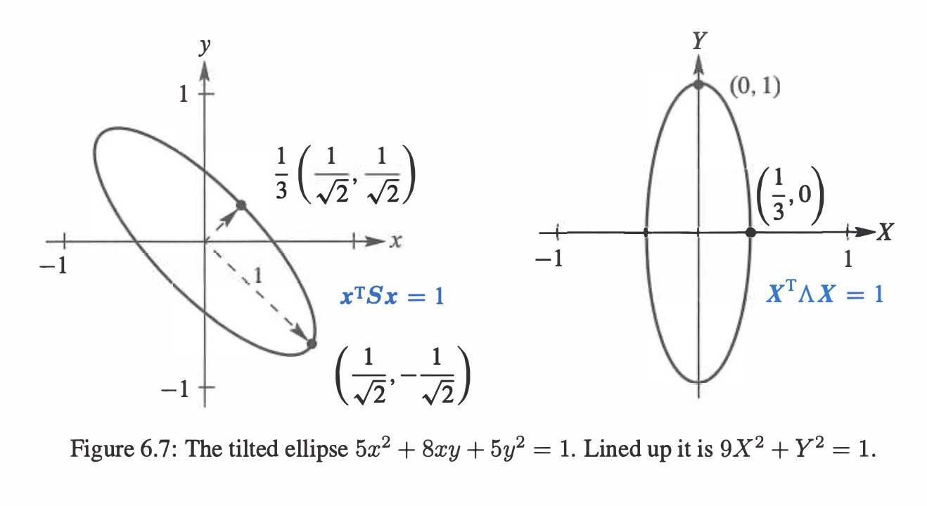
The tilted ellipse $ax^2 + 2bxy + cy^2 = 1$
$\to \begin{bmatrix}x & y\end{bmatrix}\begin{bmatrix}a & b \\ b & c\end{bmatrix}\begin{bmatrix}x \\ y\end{bmatrix} = 1 \\ \to x^TSx = 1 \to S = \begin{bmatrix}a & b \\ b & c\end{bmatrix}$
Example: Find the axes of this tilted ellipse $5x^2 + 8xy + 5y^2 = 1$.
$\to S = \begin{bmatrix}5 & 4 \\ 4 & 5\end{bmatrix}\to \lambda_1 = 1, \lambda_2 = 9\to eigenvector\space \begin{bmatrix}1\\1\end{bmatrix}, \begin{bmatrix}1\\-1\end{bmatrix}\\\to\begin{bmatrix}5 & 4 \\ 4& 5\end{bmatrix} = \frac{1}{\sqrt{2}}\begin{bmatrix}1 & 1\\1 & -1\end{bmatrix}\begin{bmatrix}9 & 0\\0 &1\end{bmatrix}\frac{1}{\sqrt{2}}\begin{bmatrix}1 & 1\\1 & -1\end{bmatrix} = Q\varLambda Q^T$

Now multiply by $[x\space y]$ on the left and$[x\space y]^T$on the right to get $x^TSx=(x^TQ)\varLambda(Q^Tx)$
$x^TSx = \text{sum of squares} \to 5x^2 + 8xy + 5y^2 = 9(\frac{x+y}{\sqrt{2}})^2 + 1(\frac{x - y}{\sqrt{2}})^2$

The coefficients are the eigenvalues 9 and 1 from $\varLambda$. Inside the squares are the eigenvectors $q_1 =(1,1)/\sqrt{2}$ and $q_2 =(1,-1)/\sqrt{2}$.
The axes of the tilted ellipse point along those eigenvectors. This explains why $S = Q\varLambda Q^T$ is called the “principal axis theorem”—it displays the axes.

$S= Q\varLambda Q^T$ is positive definite when all $\lambda_i > 0$. The graph of $x^TSx = 1$ is an ellipse
$\text{Ellipse } \begin{bmatrix}x & y\end{bmatrix}Q\varLambda Q^T\begin{bmatrix}x\\y\end{bmatrix} = \begin{bmatrix}X&Y\end{bmatrix}\varLambda\begin{bmatrix}X\\Y\end{bmatrix} = \lambda_1X^2 + \lambda_2Y^2 = 1$
The axes point along eigenvectors of $S$. The half-lengths are $\frac{1}{\sqrt{\lambda_1}}$ and $\frac{1}{\sqrt{\lambda_2}}$

Singular Value Decomposition (SVD)

Image Processing by Linear Algebra

1. The singular value theorem for $A$ is the eigenvalue theorem for $A^TA$ and $AA^T$.

A has two sets of singular vectors (the eigenvectors of $A^TA$ and $AA^T$). There is one set of positive singular values (because $A^TA$ has the same positive eigenvalues as $AA^T$). $A$ is often rectangular, but $A^TA$ and $AA^T$ are square, symmetric, and positive semidefinite.

2. The Singular ValueDecomposition (SVD) separates any matrix into simple pieces.

Each piece is a column vector times a row vector.

3. Use the eigenvectors $u$ of $AA^T$ and the eigenvectors $v$ of $A^TA$.

Since $AA^T$ and $A^TA$ are automatically symmetric (but not usually equal!) the $u$'s will be one orthogonal set and the eigenvectors $v$ will be another orthogonal set. We can and will make them all unit vectors: $||u_i|| = 1$ and $||v_i|| = 1$. Then our rank 2 matrix will be $A = \sigma_1u_1v_1^T + \sigma_2u_2v_2^T$ The size of those numbers $\sigma_1$ and $\sigma_2$ will decide whether they can be ignored in compression. We keep larger $\sigma$'s, we discard small $\sigma$'s.
The $u$'s from the SVD are called left singular vectors (unit eigenvectors of $AA^T$ ).
The $v$'s from the SVD are called right singular vectors (unit eigenvectors of $A^TA$ ).
The $\sigma$'s are singular values, square roots$(\sqrt \lambda)$ of the equal eigenvalues of $AA^T$ and $A^TA$
$\text{Choices from the SVD: }\hspace{2em} AA^Tu_i = \sigma_i^2u_i \hspace{1em} A^TAv_i = \sigma_i^2v_i \hspace{1em} Av_i = \sigma_iu_i$

Bases and Matrices in the SVD

A is any $m$ by $n$ matrix, square or rectangular. Its rank is $r$. We will diagonalize this $A$, but not by $X^{-1}AX$. The eigenvectors in $X$ have three big problems:

• They are usually not orthogonal,
• there are not always enough eigenvectors,
• and $Ax = \lambda x$ requires $A$ to be a square matrix.

The singular vectors of $A$ solve all those problems in a perfect way.

1. The SVD produces orthonormal basis of $v$'s and $u$'s for the four fundamental subspaces.

There are two sets of singular vectors, $u$'s and $v$'s. The $u$'s are in $R^m$ and the $v$'s are in $R^n$. They will be the columns of an $m$ by $m$ matrix $U$ and an $n$ by $n$ matrix $V$
The $u$'s and $v$'s give bases for the four fundamental subspaces:

$u_1,\cdots,u_r$ is an orthonormal basis for the column space
$u_{r+1},\cdots,u_m$ is an orthonormal basis for the left nullspace $N(A^T)$
$v_1,\cdots,v_r$ is an orthonormal basis for the row space
$v_{r+1},\cdots,v_n$ is an orthonormal basis for the nullspace $N(A)$.

More than just orthogonality, these basis vectors diagonalize the matrix A:

$\text{A is diagonalized} \hspace{1em} Av_1 = \sigma_1u_1 \hspace{1em} Av_2 = \sigma_2u_2 \hspace{1em}\cdots\hspace{1em} Av_r = \sigma_ru_r$

Those singular values $\sigma_1$ to $\sigma_r$ will be positive numbers: $\sigma_i$ is the length of $Av_i$. The $\sigma$'s go into a diagonal matrix that is otherwise zero. That matrix is $\sum$.

Since the $u$'s are orthonormal, the matrix $U_r$ with those $r$ columns has $U_r^TU_r = I$. Since the $v$'s are orthonormal, the matrix $V_r$ has $V_r^TV_r = I$. Then the equations $Av_i=\sigma_iu_i$ tell us column by column that $AV_r =U_r\sum_r$

$AV_r = U_r\sum_r \to A\begin{bmatrix}v_1 & \cdots & v_r\end{bmatrix} = \begin{bmatrix}u_1 & \cdots & u_r\end{bmatrix} \begin{bmatrix}\sigma_1 & & \\ & \ddots & \\ & & \sigma_r\end{bmatrix}$

This is the heart of the SVD, but there is more. Those $v$'s and $u$'s account for the row space and column space of $A$. We have $n - r$ more $v$'s and $m - r$ more $u$'s, from the nullspace $N(A)$ and the left nullspace $N(A^T)$. They are automatically orthogonal to the first $v$'s and $u$'s (because the whole nullspaces are orthogonal). We now include all the $v$'s and $u$'s in $V$ and $U$, so these matrices become square. We still have $AV = U\sum$.

$AV = U\sum \to A\begin{bmatrix}v_1 & \cdots & v_r & \cdots & v_n\end{bmatrix} = \begin{bmatrix}u_1 & \cdots & u_r & \cdots & u_m\end{bmatrix} \begin{bmatrix}\sigma_1 & & & \\ & \ddots & & \\ & & \sigma_r & \\ & & & \end{bmatrix}$

The new $\sum$ is $m$ by $n$. It is just the $r$ by $r$ matrix inequation above with $m-r$ extra zero rows and $n - r$ new zero columns. The real change is in the shapes of $U$ and $V$. Those are square matrices and $V^{-1}= V^T$ . So $AV= U\sum$ becomes $A= U\sum V$ . This is the Singular Value Decomposition.

$\text{SVD}\hspace{1em} A = U\sum V^T = u_1\sigma_1v_1^T + \cdots + u_r\sigma_rv_r^T$

It’s is crucial that each $\sigma_i^2$ is an eigenvalue of $A^TA$ and also $AA^T$. When we put the singular values in descending order, $\sigma_1 \ge \sigma_2\ge \cdots \sigma_ r > 0$, the splitting in equation above gives the $r$ rank-one pieces of $A$ in order of importance.

Example, Find the matrices $U, \sum, V$ for $A = \begin{bmatrix}3 & 0 \\ 4 & 5\end{bmatrix}$

$\to A^TA = \begin{bmatrix}25 & 20 \\ 20 & 25\end{bmatrix}, AA^T = \begin{bmatrix}9 & 12 \\ 12 & 41\end{bmatrix}\to \lambda_1 = 45, \lambda_2 = 5 \\ \to \sigma_1^2 = \lambda_1 = 45, \sigma_2^2 = \lambda_2 = 5 \\ \to \text{eigenvectors for }A^TA, v_1 = \frac{1}{\sqrt{2}}\begin{bmatrix} 1 \\ 1\end{bmatrix}, v_2 = \frac{1}{\sqrt{2}}\begin{bmatrix} -1 \\ 1\end{bmatrix} \\ \to u_i = \frac{Av_i}{\sigma_i}\to u_1 = \frac{1}{\sqrt{10}}\begin{bmatrix} 1 \\ 3\end{bmatrix}, u_2 = \frac{1}{\sqrt{10}}\begin{bmatrix} -3 \\ 1\end{bmatrix} \\ \to U = \frac{1}{\sqrt{10}}\begin{bmatrix} 1 & -3 \\ 3&1\end{bmatrix}, \sum = \begin{bmatrix} \sqrt{45} & \\ & \sqrt{5}\end{bmatrix}, V = \frac{1}{\sqrt{2}}\begin{bmatrix} 1 & -1 \\ 1&1\end{bmatrix}\\ \to AV = U\sum \to A = U\sum V^{-1} \to A = \sigma_1u_1v_1^T + \sigma_2u_2v_2^T$

Singular Vectors of $A$ and Eigenvectors of $S = A^TA$

$\text{Symmetric S}\hspace{1em} S = Q\varLambda Q^T = \lambda_1q_1q_1^T + \lambda_2q_2q_2^T + \cdots + \lambda_rq_rq_r^T \\ \text{Anymatrix A}\hspace{1em} A = U\sum V^T = \sigma_1u_1v_1^T + \sigma_2u_2v_2^T + \cdots + \sigma_ru_rv_r^T$

Principal Component Analysis (PCA by the SVD)

This section explains a major application of the SVD to statistics and data analysis.
PCA gives a way to understand a data plot in dimension $m =$ the number of measured variables (here age and height). Subtract average age and height ($m = 2$ for $n$ samples) to center the $m$ by $n$ data matrix A. The crucial connection to linear algebra is in the singular values and singular vectors of $A$. Those come from the eigenvalues $\lambda=\sigma^2$ and the eigenvectors $u$ of the sample covariance matrix $S = AA^T/(n - 1)$.

1. The total variance in the data is the sum of all eigenvalues and of sample variances $s^2$ : $\text{Total variance T} = \sigma_1^2 + \cdots + \sigma_m^2= s_1^2 + \cdots + s_m^2 = \text{trace (diagonal sum)}$
2. The first eigenvector $u_1$ of $S$ points in the most significant direction of the data. That direction accounts for (or explains) a fraction $\sigma_1^2/T$ of the total variance.
3. The next eigenvector $u_2$ (orthogonal to $u_1$) accounts for a smaller fraction $\sigma_2^2/T$.
4. Stop when those fractions are small. You have the $R$ directions that explain most of the data. The $n$ data points are very near an R-dimensional subspace with basis $u_1$ to $U_R$ — These $u$'s are the principal components in $m-dimensional$ space.
5. $R$ is the “effective rank” of $A$. The true rank $r$ is probably $m$ or $n$ : full rank matrix.

matrix-analysis

Reference

• Introduction to linear algebra by glbert strang
• Matrix Analysis & Applied Linear Algebra