Pattern Recognition And Machine Learning(模式识别&机器学习)

introduction

keywords

• supervised learning
  Supervised learning, in the context of artificial intelligence (AI) and machine learning, is a type of system in which both input and desired output data are provided. Input and output data are labelled for classification to provide a learning basis for future data processing.

• unsupervised learning
  opposite of supervised learning

• classification
  Cases such as the digit recognition example, in which the aim is to assign each input vector to one of a finite number of discrete categories

• reinforcement learning
  Reinforcement learning is where a system, or agent, tries to maximize some measure of reward while interacting with a dynamic environment. If an action is followed by an increase in the reward, then the system increases the tendency to produce that action.

• regression
  If the desired output consists of one or more continuous variables, then the task is called regression

• error function

• over-fitting

• generalization

• credit assignment

• regularization

• maximum likelihood

• Polynomial Curve Fitting

• shrinkage methods

• ridge regression

• weight decay

• Minkowski loss

• differential entropy

In other pattern recognition problems, the training data consists of a set of input vectors x without any corresponding target values. The goal in such unsupervised learning problems may be to discover groups of similar examples within the data, where it is called clustering, or to determine the distribution of data within the input space, known as density estimation, or to project the data from a high-dimensional space down to two or three dimensions for the purpose of visualization.

Polynomial Curve Fitting

suppose that we are given a training set comprising N observations of x, written

$\mathbf x \equiv (x_1, ..., x_n)^\top$

together with corresponding observations of the values of t ,denoted

$\mathbf t \equiv (t_1, ..., t_n)^\top$

we shall fit the data using a polynomial function of the form

$y(x, w) = w_0 + w_1x + w_2x^2 + ... + w_nx^n= \sum_{j=0}^{n} w_jx^j \tag{1.1.1}$

where n is the order of the polynomial, and $x^j$ denotes x raised to the power of j.
The polynomial coefficients $w_0$, … , $w_n$ are collectively denoted by the vector w.
Note that, although the polynomial function $y(x, w)$ is a nonlinear function of x, it is a linear function of the coefficients w.

The values of the coefficients will be determined by fitting the polynomial to the training data. This can be done by minimizing an error function that measures the misfit between the function $y(x, w)$, for any given value of w, and the training set data points.

One simple choice of error function, which is widely used, is given by the sum of the squares of the errors between the predictions $y(x_n, w)$ for each data point $x_n$ and the corresponding target values $t_n$, so that we minimize

$\displaystyle E(w) = \frac{1}{2} \sum_{n=1}^N \{y(x_n, w) - t_n\}^2 \tag{1.1.2}$

where the factor of 1/2 is included for later convenience. We can solve the curve fitting problem by choosing the value of w for which E(w) is as small as possible.

It is sometimes more convenient to use the root-mean-square

$\displaystyle E_{RMS} = \sqrt\frac{2E(w^*)}{N} \tag{1.1.3}$

in which the division by N allows us to compare different sizes of data sets on an equal footing, and the square root ensures that $E_{RMS}$ is measured on the same scale (and in the same units) as the target variable t.

there is something rather unsatisfying about having to limit the number of parameters in a model according to the size of the available training set. It would seem more reasonable to choose the complexity of the model according to the complexity of the problem being solved. We shall see that the least squares approach to finding the model parameters represents a specific case of maximum likelihood, and that the over-fitting problem can be understood as a general property of maximum likelihood. By adopting a Bayesian approach, the over-fitting problem can be avoided. We shall see that there is no difficulty from a Bayesian perspective in employing models for which the number of parameters greatly exceeds the number of data points. Indeed, in a Bayesian model the effective number of parameters adapts automatically to the size of the data set

For the moment, however, it is instructive to continue with the current approach and to consider how in practice we can apply it to data sets of limited size where we may wish to use relatively complex and flexible models. One technique that is often used to control the over-fitting phenomenon in such cases is that of regularization, which involves adding a penalty term to the error function (1.1.2) in order to discourage the coefficients from reaching large values. The simplest such penalty term takes the form of a sum of squares of all of the coefficients, leading to a modified error function of the form

$\displaystyle \text{\~{E}(w)} \equiv \frac{1}{2}\sum_{n=1}^{N}\{y(x_n, w) - t_n\}^2 + \frac{\lambda}{2}||w||^2 \tag{1.1.4}$

where $||w||^2 \equiv\bf{w}^\top\bf{w}\rm{=w_0^2 + w_1^2 + ... + w_m^2}$, and the coefficient λ governs the relative importance of the regularization term compared with the sum-of-squares error term.

Note that often the coefficient w0 is omitted from the regularizer because its inclusion causes the results to depend on the choice of origin for the target variable (Hastie et al., 2001), or it may be included but with its own regularization coefficient.

Again, the error function in (1.1.4) can be minimized exactly in closed form. Techniques such as this are known in the statistics literature as shrinkage methods because they reduce the value of the coefficients. The particular case of a quadratic regularizer is called ridge regres- sion (Hoerl and Kennard, 1970). In the context of neural networks, this approach is known as weight decay.

Probability Theory

Probability densities

A key concept in the field of pattern recognition is that of uncertainty. It arises both through noise on measurements, as well as through the finite size of data sets. Prob- ability theory provides a consistent framework for the quantification and manipula- tion of uncertainty and forms one of the central foundations for pattern recognition. Combined with decision theory, it allows us to make optimal predictions given all the information available to us, even though that information may be incomplete or ambiguous.

The probability that X will take the value $x_i$ and Y will take the value $y_j$ is written $p(X = x_i,Y = y_j)$ and is called the joint probability of X = $x_i$ and $Y = y_j$ . It is given by the number of points falling in the cell i,j as a fraction of the total number of points, and hence

$p(X = x_i, Y = y_j) = \frac{n_{ij}}{N} \tag{1.2.1}$

Here we are implicitly considering the limit $N \to \infty$. Similarly, the probability that X takes the value $x_i$ irrespective of the value of Y is written as $p(X = x_i)$ and is given by the fraction of the total number of points that fall in column i, so that

$p(X = x_i) = \frac{c_i}{N} \tag{1.2.2}$

Because the number of instances in column i is just the sum of the number of instances in each cell of that column, we have $c_i = \sum_jn_{ij}$ nij and therefore, from (1.2.1) and (1.2.2), we have

$\displaystyle p(X = x_i) = \sum_{j=1}^Lp(X = x_i, Y = y_j) \tag{1.2.3}$

which is the sum rule of probability. Note that $p(X = x_i)$ is sometimes called the marginal probability, because it is obtained by marginalizing, or summing out, the other variables (in this case Y ).

If we consider only those instances for which $X = x_i$, then the fraction of such instances for which $Y = y_j$ is written $p(Y = yj|X = xi)$ and is called the conditional probability of $Y = y_j$ given $X = x_i$. It is obtained by finding the fraction of those points in column i that fall in cell i,j and hence is given by

$p(Y = y_j|X = x_i) = \frac{n_{ij}}{c_i} \tag{1.2.4}$

From (1.2.1), (1.2.2), (1.2.4) we can then derive the following relationship

$p(X = x_i, Y = y_j) = \frac{n_{ij}}{N} = \frac{n_{ij}}{c_i} \cdot \frac{c_i}{N} = p(Y = y_j|X = x_i) \cdot p(X = x_i) \tag{1.2.5}$

which is the product rule of probability.

two fundamental rules of probability theory in the following form.

• sum rule

$\displaystyle p(X) = \sum_Yp(X,Y) \tag{1.2.6}$

• product rule

$\displaystyle p(X,Y) = p(Y|X) \cdot p(X) \tag{1.2.7}$

From the product rule, together with the symmetry property $p(X, Y ) = p(Y, X)$, we immediately obtain the following relationship between conditional probabilities

$p(Y|X) = \frac{p(X|Y) \cdot p(Y)}{p(X)} \tag{1.2.8}$

which is called Bayes’ theorem and which plays a central role in pattern recognition and machine learning.

Using the sum rule, the denominator in Bayes’ theorem can be expressed in terms of the quantities appearing in the numerator

$p(X) = \sum_Yp(X|Y) \cdot p(Y) \tag{1.2.9}$

We can view the denominator in Bayes’ theorem as being the normalization constant required to ensure that the sum of the conditional probability on the left-hand side of (1.2.8) over all values of Y equals one.

Probability densities

As well as considering probabilities defined over discrete sets of events, we also wish to consider probabilities with respect to continuous variables. If the probability of a real-valued variable x falling in the interval $(x, x + δx)$ is given by $p(x)δx$ for $δx \to 0$, then $p(x)$ is called the probability density over x. The probability that x will lie in an interval $(a, b)$ is then given by

$p(x \in (a, b)) = \int_{a}^{b}p(x)dx\tag{1.2.10}$

Because probabilities are nonnegative, and because the value of x must lie somewhere on the real axis, the probability density p(x) must satisfy the two conditions

• probabilities are nonnegativ

$p(x) \ge 0 \tag{1.2.11}$

• integrad of probability density is 1

$\int_{-\infty }^{\infty}p(x)dx = 1 \tag{1.2.12}$

Under a nonlinear change of variable, a probability density transforms differently from a simple function, due to the Jacobian factor. For instance, if we consider a change of variables $x = g(y)$, then a function $f(x)$ becomes $f(y) = f(g(y))$. Now consider a probability density $p_x(x)$ that corresponds to a density $p_y(y)$ with respect to the new variable y, where the suffices denote the fact that $p_x(x)$ and $p_y(y)$ are different densities. Observations falling in the range $(x, x + δx)$ will, for small values of $δx$, be transformed into the range $(y, y + δy)$ where $px(x)δx \backsimeq py(y)δy$, and hence

$p_y(y) = p_x(x) |\frac{dx}{dy}| \\ \hspace{4.2em} = p_x(g(y)) |g^{'}(y)| \tag{1.2.13}$

One consequence of this property is that the concept of the maximum of a probability density is dependent on the choice of variable.
The probability that x lies in the interval $(−\infty,z)$ is given by the cumulative distribution function(CDF) defined by

$P(z) = \int_{\infty}^zp(x)dx \tag{1.2.14}$

which satisfies $P^{'}(x) = p(x)$

If we have several continuous variables $x_1 , . . . , x_D$ , denoted collectively by the vector x, then we can define a joint probability density $p(x) = p(x_1 , . . . , x_D )$ such that the probability of x falling in an infinitesimal volume $δx$ containing the point x is given by $p(x)δx$. This multivariate probability density must satisfy $p(x) \ge 0$ and $\int p(x)dx = 1$ in which the integral is taken over the whole of x space. We can also consider joint probability distributions over a combination of discrete and continuous variables.

Note that if x is a discrete variable, then $p(x)$ is sometimes called a probability mass function because it can be regarded as a set of ‘probability masses’ concentrated at the allowed values of x.

The sum and product rules of probability, as well as Bayes’ theorem, apply equally to the case of probability densities, or to combinations of discrete and continuous variables. For instance, if x and y are two real variables, then the sum and product rules take the form

• sum rule

$\displaystyle p(x) = \int p(x,y)dy \tag{1.2.15}$

• product rule

$\displaystyle p(x,y) = p(y|x) p(x) \tag{1.2.16}$

Expectations and covariances

One of the most important operations involving probabilities is that of finding weighted averages of functions. The average value of some function $f(x)$ under a probability distribution $p(x)$ is called the expectation of $f(x)$ and will be denoted by $E[f]$.

• For a discrete distribution, the average is weighted by the relative probabilities of the different values of x

$\displaystyle E[f] = \sum_x p(x)f(x) \tag{1.2.17}$

• For continuous variables, expectations are expressed in terms of an integration with respect to the corresponding probability density

$\displaystyle E[f] = \int p(x)f(x)dx \tag{1.2.18}$

In either case, if we are given a finite number N of points drawn from the probability distribution or probability density, then the expectation can be approximated as a finite sum over these points

$\displaystyle E[f] \backsimeq \frac{1}{N}\sum_{n=1}{N}f(x_n) \tag{1.2.19}$

Sometimes we will be considering expectations of functions of several variables, in which case we can use a subscript to indicate which variable is being averaged over, so that for instance $E_x[f(x,y)]$ denotes the average of the function $f(x, y)$ with respect to the distribution of x. Note that $E_x[f(x,y)]$ will be a function of y.

We can also consider a conditional expectation with respect to a conditional distribution, so that

$\displaystyle E_x[f|y] = \sum_xp(x|y) f(x) \tag{1.2.20}$

The variance of f(x) is defined by

$\displaystyle var[f] = E[(f(x) - E[f(x)])^2 ] \tag{1.2.21}$

Expanding out the square, we see that the variance can also be written in terms of the expectations of $f(x)$ and $f(x)^2$

$\displaystyle var[f] = E[f(x)^2] - E[f(x)]^2 \tag{1.2.22}$

for variabce of one variable x
$\displaystyle var[x] = E[x^2] - E[x]^2$

for random variables x and y, the covariance is defined by
$\displaystyle cov[x,y] = E_{x,y}[\{x - E[x]\}\{y - E[y]\}] = E_{x,y}[xy] - E[x]E[y]$

for two vectors of random variables $\mathbf x$ and $\mathbf y$, the covariance is a matrix
$\displaystyle cov[\mathbf x, \mathbf y] = E_{\mathbf x, \mathbf y}[\{\mathbf x - E[\mathbf x]\}\{\mathbf y^\top - E[\mathbf y^\top]\}] = E_{\mathbf x, \mathbf y}[\mathbf {xy^\top}] - E[\mathbf x]E[\mathbf y^\top]$

Bayesian probabilities

So far, we have viewed probabilities in terms of the frequencies of random, repeatable events. We shall refer to this as the classical or frequentist interpretation of probability. Now we turn to the more general Bayesian view, in which probabilities provide a quantification of uncertainty.

we can adopt a similar approach when making inferences about quantities such as the parameters $\mathbf w$ in the polynomial curve fitting example. We capture our assumptions about $\mathbf w$, before observing the data, in the form of a prior probability distribution $p(w)$. The effect of the observed data $D = \{t_1, . . . , t_N \}$ is expressed through the conditional probability $p(D|w)$, how this can be represented explicitly. Bayes’ theorem, which takes the form

$\displaystyle p(\mathbf w|D) = \frac{p(D|\mathbf w)p(\mathbf w)}{p(D)} \tag{1.2.23}$

then allows us to evaluate the uncertainty in $\mathbf w$ after we have observed D in the form of the posterior probability $p(w|D)$

The quantity $p(D|w)$ on the right-hand side of Bayes’ theorem is evaluated for the observed data set $D$ and can be viewed as a function of the parameter vector $\mathbf w$, in which case it is called the likelihood function.It expresses how probable the observed data set is for different settings of the parameter vector $\mathbf w$.

Note that the likelihood is not a probability distribution over $\mathbf w$, and its integral with respect to $\mathbf w$ does not (necessarily) equal one.

Given this definition of likelihood, we can state Bayes’ theorem in words: $posterior \propto likelihood \times prior$ where all of these quantities are viewed as functions of $\mathbf w$.

The denominator in (1.2.23) is the normalization constant, which ensures that the posterior distribution on the left-hand side is a valid probability density and integrates to one. Indeed, integrating both sides of (1.2.23) with respect to $\mathbf w$, we can express the denominator in Bayes’ theorem in terms of the prior distribution and the likelihood function

$\displaystyle p(D) = \int p(D|\mathbf w)p(\mathbf w)d\mathbf w \tag{1.2.24}$

In both the Bayesian and frequentist paradigms, the likelihood function $p(D|\mathbf w)$ plays a central role. However, the manner in which it is used is fundamentally different in the two approaches. In a frequentist setting, $\bf w$ is considered to be a fixed parameter, whose value is determined by some form of ‘estimator’, and error bars on this estimate are obtained by considering the distribution of possible data sets $D$. By contrast, from the Bayesian viewpoint there is only a single data set $D$ (namely the one that is actually observed), and the uncertainty in the parameters is expressed through a probability distribution over $\mathbf w$.

A widely used frequentist estimator is maximum likelihood, in which $\mathbf w$ is set to the value that maximizes the likelihood function $p(D|\mathbf w)$. This corresponds to choosing the value of $\mathbf w$ for which the probability of the observed data set is maximized. In the machine learning literature, the negative log of the likelihood function is called an error function. Because the negative logarithm is a monotonically decreasing function, maximizing the likelihood is equivalent to minimizing the error.

The Gaussian distribution

For the case of a single real-valued variable x, the Gaussian distribution is defined by

$\mathcal{N}(x|\mu, \sigma^2) = \frac{1}{\sqrt{2\pi}\sigma} exp(-\frac{(x - \mu)^2}{2\sigma^2}) \tag{1.2.25}$

which is governed by two parameters: $μ$, called the mean, and $σ2$, called the variance. The square root of the variance, given by $σ$, is called the standard deviation, and the reciprocal of the variance, written as $β = 1/σ^2$, is called the precision.

From the form of (1.2.25) we see that the Gaussian distribution satisfies $\mathcal{N}(x|\mu, \sigma^2) > 0$. Also it is straightforward to show that the Gaussian is normalized, so that

$\int _{\infty}^\infty \mathcal{N}(x|\mu, \sigma^2)dx = 1 \tag{1.2.26}$

$E(x) = \int_{-\infty}^{+\infty}\mathcal{N}(x|\mu, \sigma^2)xdx = \mu \tag{1.2.27}$

$E(x^2) = \int_{-\infty}^{+\infty}\mathcal{N}(x|\mu, \sigma^2)x^2dx = \mu^2 + \sigma^2 \tag{1.2.28}$

$Var(x) = E(x^2) - E[x]^2 = \sigma^2 \tag{1.2.29}$

Proof the form (1.2.26-1.2.29) with standard gaussian distribution($\mu = 0, \sigma = 1$), the common gaussian distribution $(\mu, \sigma)$ can be linear transform of the standard one.

gaussian distribution $\displaystyle f(x|\mu, \sigma^2) = \frac{1}{\sqrt{2\pi }\sigma }exp(-\frac{(x-\mu)^{2}}{2\sigma^{2}})$
standard gaussian distribution $\displaystyle f(x) = \frac{1}{\sqrt{2\pi } }exp(-\frac{x^{2}}{2})$
let $\Iota = f(x)$ then
$\Iota = \int_{-\infty }^{+\infty }\frac{1}{\sqrt{2\pi } }exp(-\frac{x^{2}}{2})dx = \int_{-\infty }^{+\infty }\frac{1}{\sqrt{2\pi } }exp(-\frac{y^{2}}{2})dy$
$\Iota^2 = \int_{-\infty }^{+\infty }\frac{1}{\sqrt{2\pi } }exp(-\frac{x^{2}}{2})dx\int_{-\infty }^{+\infty }\frac{1}{\sqrt{2\pi } }exp(-\frac{y^{2}}{2})dy = \frac{1}{2\pi}\int_{-\infty }^{+\infty }\int_{-\infty }^{+\infty }exp(-\frac{(x^{2}+y^{2})}{2})dxdy$
let $x = r\cos\theta, y = r\sin\theta$
so $dxdy = abs(jacobian) * drd\theta$
where $jacobian = \begin{vmatrix} cos\theta & sin\theta \\ -rsin\theta & rcos\theta \end{vmatrix}$
then $abs(jacobian) = abs(rcos^2\theta + rsin^2\theta) = r$
then $dxdy = abs(jacobian) * drd\theta = rdrd\theta$
then $\Iota^2 = \frac{1}{2\pi}\int_{-\infty}^{+\infty}\int_{-\infty}^{+\infty}exp(-\frac{(x^{2}+y^{2})}{2})dxdy = \frac{1}{2\pi}\int_{0}^{2\pi}\int_{0}^{+\infty }exp(-\frac{r^{2}}{2})rdrd\theta = \int_{0}^{+\infty }exp(-\frac{r^{2}}{2})rdr$
image that $t = \frac{r^{2}}{2}$
then $\Iota^2 = \int_{0}^{+\infty }exp(-\frac{r^{2}}{2})rdr = \int_{0}^{+\infty }exp(-t)dt = 1$
clearly $\Iota = \int_{-\infty }^{+\infty }\frac{1}{\sqrt{2\pi } }exp(-\frac{x^{2}}{2})dx = \int_{-\infty }^{+\infty }\frac{1}{\sqrt{2\pi } }exp(-\frac{y^{2}}{2})dy = 1$
as the normal gaussion distribution $f(x)$ satisfies

translate rule: $\int_{-\infty }^{+\infty }f(x)dx =\int_{-\infty }^{+\infty }f(x-c)dx$
scale rule: $\hspace{1em} \int_{-\infty }^{+\infty }f(x)dx =\frac{1}{a}\int_{-\infty }^{+\infty }f(\frac{x}{a})dx$
so the integral of any gaussion distribution density function equals 1
$\int_{-\infty}^{\infty}\frac{1}{\sqrt{2\pi\sigma^2}}\exp\left\{-\frac{(x-\mu)^2}{2\sigma^2}\right\}dx=1$
mean of guassion distribution：
gaussian distribution function defined $f(x|\mu, \sigma^2) = \frac{1}{\sqrt{2\pi }\sigma }exp(-\frac{(x-\mu)^{2}}{2\sigma^{2}})$
where $\mu$ and $\sigma$ are two parameters, with $\sigma > 0$. By definition of the mean we have
$E(x) \\ = \int_{-\infty }^{+\infty }x\frac{1}{\sqrt{2\pi }\sigma }exp(-\frac{(x-\mu)^{2}}{2\sigma^{2}})dx \\ = \int_{-\infty }^{+\infty }（x-\mu）\frac{1}{\sqrt{2\pi }\sigma }exp(-\frac{(x-\mu)^{2}}{2\sigma^{2}})dx + \int_{-\infty }^{+\infty }\mu\frac{1}{\sqrt{2\pi }\sigma }exp(-\frac{(x-\mu)^{2}}{2\sigma^{2}})dx$
let $E_1 = \int_{-\infty }^{+\infty }（x-\mu）\frac{1}{\sqrt{2\pi }\sigma }exp(-\frac{(x-\mu)^{2}}{2\sigma^{2}})dx$
let $E_2 = \int_{-\infty }^{+\infty }\mu\frac{1}{\sqrt{2\pi }\sigma }exp(-\frac{(x-\mu)^{2}}{2\sigma^{2}})dx$
clearly that, let $x^{'} = x - \mu$ then the $E_1$ is a symmetric way of $x^{'}$ that $f(x^{'}) = f(-x^{'})$
so $E_1 = 0$ and $E_2 = \mu\int_{-\infty }^{+\infty }\frac{1}{\sqrt{2\pi }\sigma }exp(-\frac{(x-\mu)^{2}}{2\sigma^{2}})dx = \mu$

$E_2 \\ = \mu\int_{-\infty }^{+\infty }\frac{1}{\sqrt{2\pi }\sigma }exp(-\frac{(x-\mu)^{2}}{2\sigma^{2}})dx \\ = \mu\int_{-\infty }^{+\infty }\frac{1}{\sqrt{2\pi }\sigma }exp(-\frac{(x-\mu)^{2}}{2\sigma^{2}})d(x - \mu)$
let $x^{''} = x - \mu$
$E_2 = \mu\int_{-\infty}^{\infty}\frac{1}{\sqrt{2\pi}\sigma}exp(-\frac{x^{''2}}{2\sigma^2})dx^{''}$
as proofed, the integral of any gaussion distribution density function equals 1, $E_2 = \mu * 1 = \mu$

variance of guassion distribution：
$Var(x) = \int_{-\infty }^{+\infty }(x-\mu)^{2}\frac{1}{\sqrt{2\pi }\sigma }exp(-\frac{(x-\mu)^{2}}{2\sigma^{2}})dx$
with the same tricks (let $y = x - \mu$) as before we have
$Var(x) = \int_{-\infty }^{+\infty }\frac{1}{\sqrt{2\pi }\sigma }exp(-\frac{y^{2}}{2\sigma^{2}})y^{2}dy = \sigma^{2}$

let $t = \frac{y}{\sqrt{2}\sigma}$
then $Var(x) = \frac{2\sigma^2}{\sqrt{\pi}} \int_{-\infty}^{+\infty} t^2 exp(-t^2)dt = \frac{2\sigma^2}{\sqrt{\pi}} \cdot \frac{\sqrt{\pi}}{2} = \sigma^2$

as $(uv)' = u' + uv'$ so $(t \space e^{-t^2})' = t' e^{-t^2} + t (e^{-t^2})' = e^{-t^2} - 2t^2e^{-t^2}$
then $t^{2}e^{-t^{2}} = \frac{1}{2} [e^{-t^2} - (t \space e^{-t^{2}})']$, integrad both side
then $\int_{-\infty}^{+\infty} t^{2}e^{-t^{2}} dt = \frac{1}{2}[ \int_{-\infty}^{+\infty} e^{-t^2}dt - \int_{-\infty}^{+\infty} (t \space e^{-t^{2}})' dt] = \frac{1}{2}( \int_{-\infty}^{+\infty} e^{-t^2}dt - t \space e^{-t^{2}}|_{-\infty}^{+\infty})$

as Hopital Rule:$\displaystyle \lim_{x\to\infty} \frac{f(x)}{g(x)} = \lim_{x\to\infty} \frac{f(x)'}{g(x)'} , \hspace{0.5em} te^{-t^2} = \frac{t}{e^{t^2}}$
then $\displaystyle \lim_{x\to+\infty}\frac{t}{e^{t^2}} = \lim_{x\to+\infty}\frac{1}{2te^{t^2}} = 0$

then $\int_{-\infty}^{+\infty} t^{2}e^{-t^{2}} dt = \frac{1}{2} \int_{-\infty}^{+\infty} e^{-t^2}dt = \frac{\sqrt{\pi}}{2}$

let $A = \int_{-\infty}^{+\infty}e^{-x^2}dx = \int_{-\infty}^{+\infty}e^{-y^2}dy$
then $A^2 = \int_{-\infty}^{+\infty}\int_{-\infty}^{+\infty}e^{-x^2 }e^{-y^2 }dxdy = \int_{-\infty}^{+\infty}\int_{-\infty}^{+\infty}e^{-(x^2 + y^2)}dxdy$
let $x = rcos\theta, y = rsin\theta$
so $dxdy = abs(jacobian) * drd\theta = rdrd\theta$
then $A^2 = \int_{0}^{2\pi}\int_{0}^{+\infty}e^{-r^2}rdrd\theta = \pi\int_{0}^{+\infty}e^{-r^2}dr^2 = \pi$
then $A = \sqrt{\pi}$

theorem for gaussion density function
$\\f(x) = \int_{-\infty}^{+\infty}\mathcal{N}(x|\mu, \sigma^2)dx = 1$
$\\E(x) = \int_{-\infty}^{+\infty}\mathcal{N}(x|\mu, \sigma^2)xdx = \mu$
$\\E(x^2) = \int_{-\infty}^{+\infty}\mathcal{N}(x|\mu, \sigma^2)x^2dx = \mu^2 + \sigma^2$
$\\Var(x) = E(x^2) - E[x]^2 = \sigma^2$

We are also interested in the Gaussian distribution defined over a D-dimensional vector x of continuous variables, which is given by

$\mathcal{N}(\mathbf x|\mathbf \mu, \mathbf{\sum}) = \frac{1}{(2\pi)^{D/2}}\frac{1}{|\mathbf{\sum}|^{1/2}}exp\{-\frac{1}{2}(\mathbf x - \mathbf \mu)^\top\mathbf{\sum}^{-1}(\mathbf x - \mathbf \mu)\} \tag{1.2.30}$

where the D-dimensional vector $μ$ is called the mean, the D × D matrix $Σ$ is called the covariance, and $|Σ|$ denotes the determinant of $Σ$.

Now suppose that we have a data set of observations $\Large \mathbf x \normalsize = (x_1, . . . , x_N )^T$, rep- resenting N observations of the scalar variable $x$. Note that we are using the typeface $\Large \mathbf x$ to distinguish this from a single observation of the vector-valued variable $(x_1,...,x_D)^T$, which we denote by $\mathbf x$. We shall suppose that the observations are drawn independently from a Gaussian distribution whose mean $μ$ and variance $σ2$ are unknown, and we would like to determine these parameters from the data set. Data points that are drawn independently from the same distribution are said to be independent and identically distributed, which is often abbreviated to i.i.d. We have seen that the joint probability of two independent events is given by the product of the marginal probabilities for each event separately. Because our data set $\Large \mathbf x$ is i.i.d., we can therefore write the probability of the data set, given $μ$ and $σ2$, in the form

$p(\mathbf x|\mu, \sigma^2) = \prod_{n=1}^{N}\mathcal{N}(x_n|\mu, \sigma^2) \tag{1.2.31}$

With the dataset sample m times randomly, get the m group data, denoted $x_1, x_2, ..., x_m$
then the likelihood function is

$\displaystyle L = L(x_1, x_2, ... x_m | \mu, \sum) = \prod_{i=1}^{m}p(x_i) = \prod_{i=1}^{m}\mathcal{N}(x_i|\mu, \sigma^2) \tag{1.2.31.1}$

One common criterion for determining the parameters in a probability distribu- tion using an observed data set is to find the parameter values that maximize the likelihood function. This might seem like a strange criterion because, from our fore- going discussion of probability theory, it would seem more natural to maximize the probability of the parameters given the data, not the probability of the data given the parameters.In fact, these two criteria are related, as we shall discuss in the context of curve fitting.

For the moment, however, we shall determine values for the unknown parameters $μ$ and $σ2$ in the Gaussian by maximizing the likelihood function (1.2.31). In practice, it is more convenient to maximize the log of the likelihood function. Because the logarithm is a monotonically increasing function of its argument, maximization of the log of a function is equivalent to maximization of the function itself. Taking the log not only simplifies the subsequent mathematical analysis, but it also helps numerically because the product of a large number of small probabilities can easily underflow the numerical precision of the computer, and this is resolved by computing instead the sum of the log probabilities.From (1.2.25) and (1.2.31), the log likelihood function can be written in the form

$ln\space p(\mathbf x|\mu, \sigma^2) = -\frac{1}{2\sigma^2}\sum_{n=1}^{N}(x_n - \mu)^2 - \frac{N}{2}ln\space\sigma^2 - \frac{N}{2}ln(2\pi) \tag{1.2.32}$

Maximizing (1.2.32) with respect to $μ$, that $\frac{\partial {ln\space p(\mathbf x|\mu, \sigma^2)}}{\partial \mu} = 0$, we obtain the maximum likelihood solution given by

$\displaystyle \mu_{ML} = \frac{1}{N}\sum_{n=1}^{N}x_n \tag{1.2.33}$

which is the sample mean, i.e., the mean of the observed values $\{x_n\}$. Similarly, maximizing (1.2.32) with respect to $σ2$, that $\frac{\partial {ln\space p(\mathbf x|\mu, \sigma^2)}}{\partial \sigma^2} = 0$ we obtain the maximum likelihood solution for the variance in the form

$\displaystyle \sigma_{ML}^2 = \frac{1}{N}\sum_{n=1}^{N}(x_n - \mu_{ML})^2 \tag{1.2.34}$

which is the sample variance measured with respect to the sample mean $μ_{ML}$

Note that we are performing a joint maximization of (1.2.32) with respect to $μ$ and $σ^2$, but in the case of the Gaussian distribution the solution for $μ$ decouples from that for $σ^2$ so that we can first evaluate (1.2.33) and then subsequently use this result to evaluate (1.2.34).

We first note that the maximum likelihood solutions $μ_{ML}$ and $σ_{ML}^2$ are functions of the data set values $x_1,...,x_N$. Consider the expectations of these quantities with respect to the data set values, which themselves come from a Gaussian distribution $μ$ and $σ^2$. It is straightforward to show that

$\displaystyle E[\mu_{ML}] = \mu \tag{1.2.35}$

$\displaystyle E[\sigma_{ML}^2] = (\frac{N-1}{N})\sigma^2 \tag{1.2.36}$

so that on average the maximum likelihood estimate will obtain the correct mean but will underestimate the true variance by a factor $(N − 1)/N$.

The intuition behind this result is that aeraged across the N data sets, the mean is correct, but the variance is systematically under-estimated because it is measured relative to the sample mean and not relative to the true mean.

From (1.2.36) it follows that the following estimate for the variance parameter is unbiased

$\tilde \sigma^2 = \frac{N}{N-1}\sigma_{ML}^2 = \frac{1}{N-1}\sum_{n=1}^{N}(x_n - \mu_{ML})^2 \tag{1.2.37}$

Note that the bias of the maximum likelihood solution becomes less significant as the number N of data points increases, and in the limit $N \to \infty$ the maximum likelihood solution for the variance equals the true variance of the distribution that generated the data. In practice, for anything other than small N, this bias will not prove to be a serious problem. However, throughout this book we shall be interested in more complex models with many parameters, for which the bias problems associated with maximum likelihood will be much more severe. In fact, as we shall see, the issue of bias in maximum likelihood lies at the root of the over-fitting problem that we encountered earlier in the context of polynomial curve fitting.
Prooved of the formula (1.2.37)

let sample meal $\bar X$, sample variance $S^2$, population mean $\mu$, populatioin variance $\sigma^2$
consider variance definition without bias $\displaystyle S^2 = \frac{1}{n}\sum_{i=1}^{n}(x_i - \bar X)^2$
$\displaystyle E(S^2)\\ = E(\frac{1}{n}\sum_{i=1}^{n}(x_i - \bar X)^2) \\ = E(\frac{1}{n}\sum_{i=1}^{n}((x_i - \mu) - (\bar X - \mu))^2)\\ = E(\frac{1}{n}\sum_{i=1}^{n}(x_i - \mu)^2 - \frac{1}{n}\sum_{i=1}^{n}2(x_i - \mu)(\bar X - \mu) + \frac{1}{n}\sum_{i=1}^{n}(\bar X - \mu)^2)\\\because \frac{1}{n}\sum_{i=1}^{n}(x_i - \mu) = \frac{1}{n}\sum_{i=1}^{n}x_i - \mu = (\bar X - \mu)\\ \therefore E(S^2)\\ = E(\frac{1}{n}\sum_{i=1}^{n}(x_i - \mu)^2 - 2(\bar X - \mu)(\bar X - \mu) + (\bar X - \mu)^2)\\ = E(\frac{1}{n}\sum_{i=1}^{n}(x_i - \mu)^2 - (\bar X - \mu)^2)\\ = E(\frac{1}{n}\sum_{i=1}^{n}(x_i - \mu)^2) - E(\bar X - \mu)^2 \le \sigma^2$
clearly, when devide n, $S^2 \le \sigma^2$, furthermore
$\displaystyle E(S^2) \\ = E(\frac{1}{n}\sum_{i=1}^{n}(x_i - \mu)^2) - E(\bar X - \mu)^2 \\ = Var(X) - Var(\bar X) \\ = \sigma^2 - \frac{1}{n}\sigma^2\\ = \frac{n - 1}{n}\sigma^2$
so when consider the bias
$\displaystyle S^2 = \frac{n}{n - 1}(\frac{1}{n}\sum_{i=1}^{n}(x_i - \bar X)^2) = \frac{1}{n - 1}\sum_{i = 1}^{n}(x_i - \bar X)^2$

Curve fitting re-visited

We have seen how the problem of polynomial curve fitting can be expressed in terms of error minimization. Here we return to the curve fitting example and view it from a probabilistic perspective, thereby gaining some insights into error functions and regularization, as well as taking us towards a full Bayesian treatment.

The goal in the curve fitting problem is to be able to make predictions for the target variable t given some new value of the input variable x on the basis of a set of training data comprising N input values $\mathbf x = (x_1 , . . . , x_N )^\top$ and their corresponding target values $\mathbf t = (t_1 , . . . , t_N )^\top$ . We can express our uncertainty over the value of the target variable using a probability distribution. For this purpose, we shall assume that, given the value of $x$, the corresponding value of $t$ has a Gaussian distribution with a mean equal to the value $y(x, \mathbf w)$ of the polynomial curve given Thus we have

$\displaystyle p(t|x, \mathbf w, \beta) = \mathcal{N}(t|y(x, \mathbf w), \beta^{-1}) \tag{1.2.38}$

where we have defined a precision parameter $\beta$ corresponding to the inverse variance of the distribution.

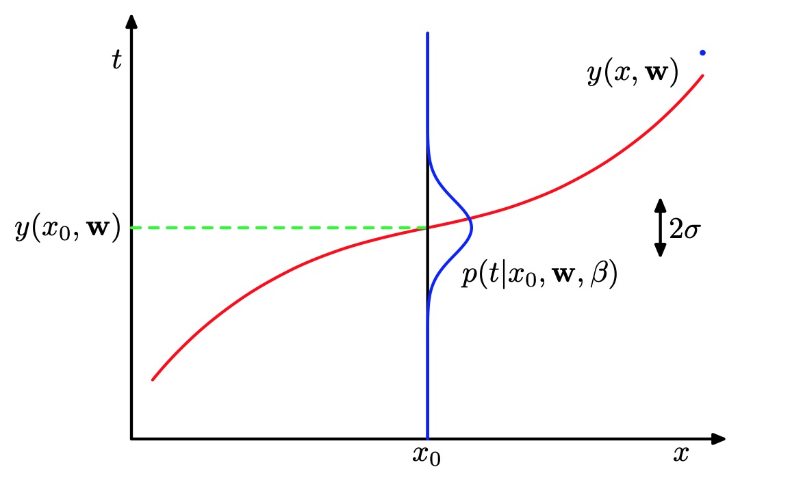
Schematic illustration of a Gaussian conditional distribution for t given x given by (1.2.25), in which the mean is given by the polynomial function $y(x,w)$, and the precision is given by the parameter $\beta$, which is related to the variance by $\beta^{-1} = \sigma^2$

We now use the training data $\{x, t\}$ to determine the values of the unknown parameters $\mathbf w$ and $\beta$ by maximum likelihood. If the data are assumed to be drawn independently from the distribution (1.2.25), then the likelihood function is given by

$\displaystyle p(\mathbf t|\mathbf x, \mathbf w, \beta) = \prod_{n=1}^{N} \mathcal{N}(t_n|y(x_n, \mathbf w), \beta^{-1}) \tag{1.2.39}$

Substituting for the form of the Gaussian distribution, given by (1.2.25), we obtain the log likelihood function in the form

$\displaystyle ln p(\mathbf t|\mathbf x, \mathbf w, \beta) = -\frac{\beta}{2}\sum_{n=1}^{N}\{y(x_n, \mathbf w) - t_n\}^2 + \frac{N}{2}ln\beta - \frac{N}{2}ln(2\pi) \tag{1.2.40}$

Consider first the determination of the maximum likelihood solution for the polynomial coefficients, which will be denoted by $\bold w_{ML}$. These are determined by maximizing (1.2.40) with respect to $\bold w$. For this purpose, we can omit the last two terms on the right-hand side of (1.2.40) because they do not depend on $\bold w$. Also, we note that scaling the log likelihood by a positive constant coefficient does not alter the location of the maximum with respect to $\bold w$, and so we can replace the coefficient β/2 with 1/2. Finally, instead of maximizing the log likelihood, we can equivalently minimize the negative log likelihood. We therefore see that maximizing likelihood is equivalent, so far as determining $\bold w$ is concerned, to minimizing the sum-of-squares error function defined by (1.1.2). Thus the sum-of-squares error function has arisen as a consequence of maximizing likelihood under the assumption of a Gaussian noise distribution.

We can also use maximum likelihood to determine the precision parameter β of the Gaussian conditional distribution. Maximizing (1.2.40) with respect to β gives

$\displaystyle \frac{1}{\beta_{ML}} = \frac{1}{N}\sum_{n=1}^{N}\{y(x_n,\mathbf w_{ML}) - t_n\}^2 \tag{1.2.41}$

Again we can first determine the parameter vector $\mathbf w_{ML}$ governing the mean and subsequently use this to find the precision $β_{ML}$ as was the case for the simple Gaussian distribution.

Having determined the parameters $\mathbf w$ and $β$, we can now make predictions for new values of $x$. Because we now have a probabilistic model, these are expressed in terms of the predictive distribution that gives the probability distribution over t, rather than simply a point estimate, and is obtained by substituting the maximum likelihood parameters into (1.2.38) to give

$\displaystyle p(t|x, \mathbf w_{ML}, \beta_{ML}) = \mathcal{N}(t|y(x, \mathbf w_{ML}), \beta_{ML}^{-1}) \tag{1.2.42}$

Now let us take a step towards a more Bayesian approach and introduce a prior distribution over the polynomial coefficients $\bold w$. For simplicity, let us consider a Gaussian distribution of the form

$p(\mathbf w|\alpha) = \mathcal{N}(\mathbf w|O, \alpha^{-1}\Iota) = (\frac{\alpha}{2\pi})^{(M + 1)/2}exp\{-\frac{\alpha}{2}\mathbf w^\top\mathbf w\} \tag{1.2.43}$

where $α$ is the precision of the distribution, and M +1 is the total number of elements in the vector $\mathbf w$ for an $M^{th}$ order polynomial. Variables such as $α$, which control the distribution of model parameters, are called hyperparameters. Using Bayes’ theorem, the posterior distribution for $\mathbf w$ is proportional to the product of the prior distribution and the likelihood function

$p(\mathbf w|\mathbf x, \mathbf t, \alpha, \beta) \propto p(\mathbf t|\mathbf x, \mathbf w, \beta) p(\mathbf w|\alpha)\tag{1.2.44}$

We can now determine $\mathbf w$ by finding the most probable value of $\mathbf w$ given the data, in other words by maximizing the posterior distribution. This technique is called maximum posterior, or simply MAP. Taking the negative logarithm of (1.2.44) and combining with (1.2.40) and (1.2.43), we find that the maximum of the posterior is given by the minimum of

$\displaystyle \frac{\beta}{2}\sum_{n=1}^{N}\{y(x_n, \mathbf w) - t_n\}^2 + \frac{\alpha}{2}\mathbf w^\top\mathbf w \tag{1.2.45}$

Thus we see that maximizing the posterior distribution is equivalent to minimizing the regularized sum-of-squares error function encountered earlier in the form (1.1.4), with a regularization parameter given by $λ = \frac{α}{β}$.

Bayesian curve fitting

Although we have included a prior distribution $p(\mathbf w|α)$, we are so far still making a point estimate of $\bold w$ and so this does not yet amount to a Bayesian treatment. In a fully Bayesian approach, we should consistently apply the sum and product rules of probability, which requires, as we shall see shortly, that we integrate over all values of $\bold w$. Such marginalizations lie at the heart of Bayesian methods for pattern recognition.

In the curve fitting problem, we are given the training data $\bold x$ and $\bold t$, along with a new test point $x$, and our goal is to predict the value of $t$. We therefore wish to evaluate the predictive distribution $p(t|x,\mathbf x,\mathbf t)$. Here we shall assume that the parameters $α$ and $β$ are fixed and known in advance (in later chapters we shall discuss how such parameters can be inferred from data in a Bayesian setting).

A Bayesian treatment simply corresponds to a consistent application of the sum and product rules of probability, which allow the predictive distribution to be written in the form

$p(t|x,\mathbf x,\mathbf t) = \int p(t|x, \mathbf w)p(\mathbf w|\mathbf x, \mathbf t)d\mathbf w \tag{1.2.46}$

Here $p(t|x, \mathbf w)$ is given by (1.2.38), and we have omitted the dependence on $α$ and $β$ to simplify the notation.Here $p(\mathbf w|\mathbf x, \mathbf t)$ is the posterior distribution over param- eters, and can be found by normalizing the right-hand side of (1.2.44). We shall see that for problems such as the curve-fitting example, this posterior distribution is a Gaussian and can be evaluated analytically. Similarly, the integration in (1.2.46) can also be performed analytically with the result that the predictive distribution is given by a Gaussian of the form

$p(t|x,\mathbf x,\mathbf t) = \mathcal{N}(t|m(x), s^2(x)) \tag{1.2.47}$

where the mean and variance are given by

mean: $\displaystyle \hspace{1em} m(x) = \beta\phi(x)^T\mathbf S\sum_{n=1}^{N}\phi(x_n)t_n$
variance: $\displaystyle s^2(x) = \beta^{-1} + \phi(x)^T\mathbf S\phi(x)$
here the matrix S is given by $\displaystyle \mathbf S^{-1} = \alpha\Iota + \beta\sum_{n=1}^{N}\phi(x_n)\phi(x)^T$

where $\Iota$ is the unit matrix, and we have defined the vector $\phi(x)$ with elements $\phi_i(x) = x_i$ for $i = 0,...,M$.

We see that the variance, as well as the mean, of the predictive distribution in (1.2.46) is dependent on $x$.

Model Selectioin

In our example of polynomial curve fitting using least squares, we saw that there was an optimal order of polynomial that gave the best generalization. The order of the polynomial controls the number of free parameters in the model and thereby governs the model complexity. With regularized least squares, the regularization coefficient $λ$ also controls the effective complexity of the model, whereas for more complex models, such as mixture distributions or neural networks there may be multiple pa- rameters governing complexity. In a practical application, we need to determine the values of such parameters, and the principal objective in doing so is usually to achieve the best predictive performance on new data. Furthermore, as well as find- ing the appropriate values for complexity parameters within a given model, we may wish to consider a range of different types of model in order to find the best one for our particular application.

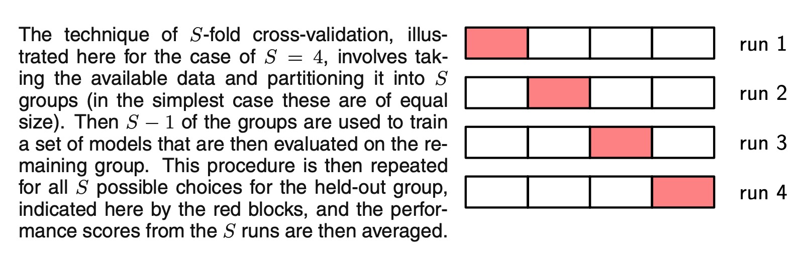
In many applications, however, the supply of data for training and testing will be limited, and in order to build good models, we wish to use as much of the available data as possible for training. However, if the validation set is small, it will give a relatively noisy estimate of predictive performance. One solution to this dilemma is to use cross-validation, which is illustrated as follow. This allows a proportion (S − 1)/S of the available data to be used for training while making use of all of the data to assess performance.When data is particularly scarce, it may be appropriate to consider the case S = N , where N is the total number of data points, which gives the leave-one-out technique.

The Curse of Dimensionality

In the polynomial curve fitting example we had just one input variable $x$. For practical applications of pattern recognition, however, we will have to deal with spaces of high dimensionality comprising many input variables. As we now discuss, this poses some serious challenges and is an important factor influencing the design of pattern recognition techniques.

Decision Thory

We have seen that how probability theory provides us with a consistent mathematical framework for quantifying and manipulating uncertainty. Here we turn to a discussion of decision theory that, when combined with probability theory, allows us to make optimal decisions in situations involving uncertainty such as those encountered in pattern recognition.

Suppose we have an input vector $\bold x$ together with a corresponding vector $\bold t$ of target variables, and our goal is to predict $t$ given a new value for $x$. For regression problems, $t$ will comprise continuous variables, whereas for classification problems it will represent class labels.The joint probability distribution $p(\bold x, \bold t)$ provides a complete summary of the uncertainty associated with these variables.

Minimizing the misclassification rate

Suppose that our goal is simply to make as few misclassifications as possible. We need a rule that assigns each value of $\bold x$ to one of the available classes. Such a rule will divide the input space into regions $R_k$ called decision regions, one for each class, such that all points in $R_k$ are assigned to class $C_k$. The boundaries between decision regions are called decision boundaries or decision surfaces. Note that each decision region need not be contiguous but could comprise some number of disjoint regions.

For the more general case of K classes, it is slightly easier to maximize the probability of being correct, which is given by

$\displaystyle p(correct) = \sum_{k=1}^{K}p(\bold x \in \bold R_k, C_k) = \sum_{k=1}^{K} \int_{\bold R_k}p(\bold x, C_k)d\bold x$

which is maximized when the regions $R_k$ are chosen such that each $\bold x$ is assigned to the class for which $p(\bold x, C_k)$ is largest.Again, using the product rule $p(\bold x, C_k)= p(C_k|\bold x)p(\bold x)$, and noting that the factor of $p(\bold x)$ is common to all terms, we see that each $\bold x$ should be assigned to the class having the largest posterior probability $p(C_k |\bold x)$.

Minimizing the expected loss

For many applications, our objective will be more complex than simply mini- mizing the number of misclassifications.
We can formalize classifier through the introduction of a loss function, also called a cost function, which is a single, overall measure of loss incurred in taking any of the available decisions or actions.Our goal is then to minimize the total loss incurred.

The optimal solution is the one which minimizes the loss function. However, the loss function depends on the true class, which is unknown. For a given input vector $\bold x$, our uncertainty in the true class is expressed through the joint probability distribution $p(\bold x, C_k)$ and so we seek instead to minimize the average loss, where the average is computed with respect to this distribution, which is given by $\displaystyle \\E[L] = \sum_{k}\sum_{j}\int_{R_j}L_{kj}p(\bold x, C_k)d\bold x$
Each $\bold x$ can be assigned independently to one of the decision regions $R_j$ .Our goal is to choose the regions $R_j$ in order to minimize the expected loss, which implies that for each $\bold x$ we should minimize $\sum_{k}L_{kj}p(\bold x, C_k)$.As before, we can use the product rule $p(\bold x,C_k) = p(C_k|\bold x)p(\bold x)$ to eliminate the common factor of p(x). Thus the decision rule that minimizes the expected loss is the one that assigns each new $\bold x$ to the class $j$ for which the quantity $\sum_{k}L_{kj}p(C_k|\bold x)$ is a minimum. This is clearly trivial to do, once we know the posterior class probabilities $p(C_k|\bold x)$.

The reject option

We have seen that classification errors arise from the regions of input space where the largest of the posterior probabilities $p(C_k |\bold x)$ is significantly less than unity, or equivalently where the joint distributions $p(\bold x, C_k)$ have comparable values. In some applications, it will be appropriate to avoid making decisions on the difficult cases in anticipation of a lower error rate on those examples for which a classification decision is made. This is known as the reject option.

Inference and decision

We have broken the classification problem down into two separate stages

the inference stage in which we use training data to learn a model for $p(C_k|\bold x)$
the decision stage in which we use these posterior probabilities to make op- timal class assignments.

To solving decision problems, find a function $f(x)$, called a discriminant function, which maps each input $\bold x$ directly onto a class label. For instance, in the case of two-class problems, $f(·)$ might be binary valued and such that $f = 0$ represents class $C_1$ and $f = 1$ represents class $C_2$. In this case, probabilities play no role, we no longer have access to the posterior probabilities $p(C_k|\bold x)$.There are many powerful reasons for wanting to compute the posterior probabilities, even if we subsequently use them to make decisions. These include:

• Minimizing risk.
  Consider a problem in which the elements of the loss matrix are subjected to revision from time to time.If we know the posterior probabilities, we can trivially revise the minimum risk decision criterion by modifying appropriately.If we have only a discriminant function, then any change to the loss matrix would require that we return to the training data and solve the classification problem afresh
• Rejectoption.
  Posterior probabilities allow us to determine a rejection criterion that will minimize the misclassification rate, or more generally the expected loss, for a given fraction of rejected data points.
• Compensating for class priors.
  A balanced data set in which we have selected equal numbers of exam- ples from each of the classes would allow us to find a more accurate model. However, we then have to compensate for the effects of our modifications to the training data. Suppose we have used such a modified data set and found models for the posterior probabilities. From Bayes’ theorem, we see that the posterior probabilities are proportional to the prior probabilities, which we can interpret as the fractions of points in each class. We can therefore simply take the posterior probabilities obtained from our artificially balanced data set and first divide by the class fractions in that data set and then multiply by the class fractions in the population to which we wish to apply the model. Finally, we need to normalize to ensure that the new posterior probabilities sum to one. Note that this procedure cannot be applied if we have learned a discriminant function directly instead of determining posterior probabilities.
• **Combining models. **
  For complex applications, we may wish to break the problem into a number of smaller subproblems each of which can be tackled by a sep- arate module.

Loss functions for regression

So far, we have discussed decision theory in the context of classification prob- lems. We now turn to the case of regression problems, such as the curve fitting example discussed earlier. The decision stage consists of choosing a specific estimate $y(\bold x)$ of the value of $t$ for each input $\bold x$.Suppose that in doing so, we incur a loss $L(t, y(\bold x))$. The average, or expected, loss is then given by

$E[L] = \int\int L(t,y(\bold x))p(\bold x, t)d\bold xdt \tag{1.3.1}$

A common choice of loss function in regression problems is the squared loss given by $L(t, y(\bold x)) = \{y(\bold x) - t\}^2$. In this case, the expected loss can be written

$E[L] = \int\int \{y(\bold x) - t\}^2p(\bold x, t)d\bold xdt \tag{1.3.2}$

Our goal is to choose y(x) so as to minimize $E[L]$. If we assume a completely flexible function $y(x)$, we can do this formally using the calculus of variations to give

$\frac{\partial E[L]}{\partial y(\bold x)} = 2\int \{y(\bold x) -t\}p(\bold x,t)dt = 0 \tag{1.3.3}$

Solving for $y(\bold x)$, and using the sum and product rules of probability, we obtain

$y(\bold x) = \frac{\int tp(\bold x, t)dt}{p(\bold x)} = \int tp(t|\bold x)dt = E[t|\bold x] \tag{1.3.4}$

which is the conditional average of $t$ conditioned on $\bold x$ and is known as the regression function.To multiple target variables represented by the vector $t$, in which case the optimal solution is the conditional average $y(\bold x) = E_t[t|\bold x]$.We can also derive this result in a slightly different way, which will also shed light on the nature of the regression problem. Armed with the knowledge that the optimal solution is the conditional expectation, we can expand the square term as follows

$\{y(\bold x) - t\}^2 = \{y(\bold x) - E[t|\bold x] + E[t|\bold x] -t\}^2 = \{y(\bold x) - E[t|\bold x]\}^2 + 2\{y(\bold x) - E[t|\bold x]\}\{E[t|\bold x] - t\} + \{E[t|\bold x] - t\}^2$

where, to keep the notation uncluttered, we use $E[t|\bold x]$ to denote $E_t[t|\bold x]$.Substituting into the loss function and performing the integral over t, we see that the cross-term vanishes and we obtain an expression for the loss function in the form

$E[L] = \int \{y(\bold x) - E[t|\bold x]\}^2p(\bold x)d\bold x + \int \{E[t|\bold x] - t\}^2p(\bold x)d\bold x \tag{1.3.5}$

The function $y(\bold x)$ we seek to determine enters only in the first term, which will be minimized when $y(\bold x)$ is equal to $E[t|\bold x]$, in which case this term will vanish. This is simply the result that we derived previously and that shows that the optimal least squares predictor is given by the conditional mean. The second term is the variance of the distribution of $t$, averaged over $\bold x$. It represents the intrinsic variability of the target data and can be regarded as noise. Because it is independent of $y(\bold x)$, it represents the irreducible minimum value of the loss function.As with the classification problem, we can either determine the appropriate prob- abilities and then use these to make optimal decisions, or we can build models that make decisions directly. Indeed, we can identify three distinct approaches to solving regression problems given, in order of decreasing complexity,by

(a). First solve the inference problem of determining the joint density $p(\bold x, t)$. Then normalize to find the conditional density $p(t|\bold x)$, and finally marginalize to find the conditional mean given by (1.3.4)
(b). First solve the inference problem of determining the conditional density $p(t|\bold x)$, and then subsequently marginalize to find the conditional mean given by (1.3.4)
©. Find a regression function $y(\bold x)$ directly from the training data.

The relative merits of these three approaches follow the same lines as for classifica- tion problems above.

The squared loss is not the only possible choice of loss function for regression. Indeed, there are situations in which squared loss can lead to very poor results and where we need to develop more sophisticated approaches. An important example concerns situations in which the conditional distribution $p(t|\bold x)$ is multimodal, as often arises in the solution of inverse problems. Here we consider briefly one simple generalization of the squared loss, called the Minkowski loss, whose expectation is given by

$E[L_q] = \int \int |y(\bold x) - t|^qp(\bold x, t)d\bold xdt \tag{1.3.6}$

which reduces to the expected squared loss for $q = 2$.The minimum of $E[L_q]$ is given by the conditional mean for $q = 2$, the conditional median for $q = 1$, and the conditional mode for $q \to 0$.

Information Theory

n this chapter, we have discussed a variety of concepts from probability theory and decision theory that will form the foundations for much of the subsequent discussion in this book. We close this chapter by introducing some additional concepts from the field of information theory, which will also prove useful in our development of pattern recognition and machine learning techniques.

We begin by considering a discrete random variable $x$ and we ask how much information is received when we observe a specific value for this variable. The amount of information can be viewed as the ‘degree of surprise’ on learning the value of $x$. If we are told that a highly improbable event has just occurred, we will have received more information than if we were told that some very likely event has just occurred, and if we knew that the event was certain to happen we would receive no information. Our measure of information content will therefore depend on the probability distribution $p(x)$, and we therefore look for a quantity $h(x)$ that is a monotonic function of the probability $p(x)$ and that expresses the information content. The form of $h(·)$ can be found by noting that if we have two events $x$ and $y$ that are unrelated, then the information gain from observing both of them should be the sum of the information gained from each of them separately, so that $h(x, y) = h(x) + h(y)$. Two unrelated events will be statistically independent and so $p(x, y) = p(x)p(y)$. From these two relationships, it is easily shown that $h(x)$ must be given by the logarithm of $p(x)$ and so we have

$h(x) = -log_2p(x) \tag{1.4.1}$

where the negative sign ensures that information is positive or zero.Note that low probability events x correspond to high information content. The choice of basis for the logarithm is arbitrary, and for the moment we shall adopt the convention prevalent in information theory of using logarithms to the base of 2.

Now suppose that a sender wishes to transmit the value of a random variable to a receiver. The average amount of information that they transmit in the process is obtained by taking the expectation of (1.4.1) with respect to the distribution $p(x)$ and is given by

$H[x] = - \sum_x p(x)log_2p(x) \tag{1.4.2}$

This important quantity is called the entropy of the random variable x.

Note that $lim_{p\to 0} p ln\space p = 0$ and so we shall take $p(x) ln\space p(x) = 0$ whenever we encounter a value for $x$ such that $p(x) = 0$.

We now show that these definitions indeed possess useful properties. Consider a random variable x having 8 possible states, each of which is equally likely. In order to communicate the value of x to a receiver, we would need to transmit a message of length 3 bits. Notice that the entropy of this variable is given by $H[x] = -8 \times \frac{1}{8}log_2\frac{1}{8} = 3 \space bits$

For a density defined over multiple continuous variables, denoted collectively by the vector $\bold x$, the differential entropy is given by

$H[\bold x] = -\int p(\bold x)ln\space p(\bold x)d\bold x \tag{1.4.3}$

In the case of discrete distributions, we saw that the maximum entropy configuration corresponded to an equal distribution of probabilities across the possible states of the variable.Let us now consider the maximum entropy configuration for a continuous variable.

Omit the proof process, the distribution that maximizes the differential entropy is the Gaussian.If we evaluate the differential entropy of the Gaussian, we obtain $H[x] = \frac{1}{2} \{1 + ln(2\pi\sigma^2)\}$

proof as follow

as prooved $\int_{-\infty}^{+\infty}e^{-x^2}dx = \sqrt\pi$

for single variant

so $H[x] \\ = -\int p(x)ln\space p(x)dx \\ = -\int \frac{1}{\sqrt{2\pi\sigma^2}}exp(-\frac{(x-\mu)^{2}}{2\sigma^{2}})ln \frac{1}{\sqrt{2\pi\sigma^2} }exp(-\frac{(x-\mu)^{2}}{2\sigma^{2}})dx \\ = - \frac{1}{\sqrt{2\pi\sigma^2}}\int exp(-\frac{(x-\mu)^{2}}{2\sigma^{2}})\{-ln(\sqrt{2\pi}\sigma) -\frac{(x-\mu)^{2}}{2\sigma^{2}}\} dx \\ = \frac{ln(\sqrt{2\pi}\sigma)}{\sqrt{2\pi\sigma^2}}\int exp(-\frac{(x-\mu)^{2}}{2\sigma^{2}})dx + \frac{1}{\sqrt{2\pi\sigma^2}}\int exp(-\frac{(x-\mu)^{2}}{2\sigma^{2}})\frac{(x-\mu)^{2}}{2\sigma^{2}} dx$
let $x' = \frac{x - \mu}{\sqrt2\sigma}$, then $H[x] \\ =\frac{ln(\sqrt{2\pi}\sigma)}{\sqrt\pi}\int_{-\infty}^{+\infty}e^{-x'^2}dx' + \frac{1}{\sqrt\pi}\int_{-\infty}^{+\infty}e^{-x'^2}x'^2dx' \\ = ln(\sqrt{2\pi}\sigma) + \frac{1}{\sqrt\pi}\int_{-\infty}^{+\infty}e^{-x'^2}x'^2dx'$
as $(uv)' = u'v + uv'$, that $x'e^{-x'^2} = e^{-x'^2} - 2x'^2e^{-x'^2}$ and $x'e^{-x'^2}$ is symmetric in $(-\infty, +\infty)$
then $H[x] \\ = ln(\sqrt{2\pi}\sigma) + \frac{1}{\sqrt\pi}\cdot -\frac{1}{2}(0 - \int_{-\infty}^{+\infty}e^{-x'^2}dx') \\ = ln(\sqrt{2\pi}\sigma) + \frac{1}{2} \\ = \frac{1}{2}(1 + ln(2\pi\sigma^2))$

for multi-variant

if $\bold x \sim \mathcal{N}(\mu, \Sigma)$, with Mahalanobis transform let $\bold y = \Sigma^{-\frac{1}{2}}[\bold x - \mu]$
then $\bold y \sim \mathcal{N}(0, \Iota_k)$, that means $y_i$ is the normalization gaussion distribution $\mathcal{N}(0,1)$
as $p(\bold x) = (2\pi)^{-\frac{k}{2}}|\Sigma|^{-\frac{1}{2}}exp[-\frac{1}{2}(\bold x - \mu)^T\Sigma^{-1}(\bold x - \mu)]$
and $\bold x = \Sigma^{\frac{1}{2}}\bold y + \mu, J = det[\frac{\partial \bold x}{\partial \bold y^T}] = |\Sigma|^{\frac{1}{2}}$
so $p(\bold y) = (2\pi)^{-\frac{k}{2}}exp[-\frac{1}{2}\bold y^T \bold y]$

so $H[\bold x] = -\int p(\bold x)ln\space p(\bold x)d\bold x \\ = -\int p(\bold x)ln\space\{(2\pi)^{-\frac{k}{2}}|\Sigma|^{-\frac{1}{2}}exp[-\frac{1}{2}(\bold x - \mu)^T\Sigma^{-1}(\bold x - \mu)]\}d\bold x \\ = -\int p(\bold x)\{ln[(2\pi)^{-\frac{k}{2}}|\Sigma|^{-\frac{1}{2}}] - \frac{1}{2}(\bold x - \mu)^T\Sigma^{-1}(\bold x - \mu) \} d\bold x \\ = ln[(2\pi)^{\frac{k}{2}}|\Sigma^{\frac{1}{2}}|] + \frac{1}{2}\int p(\bold x)[(\bold x - \mu)^T\Sigma^{-1}(\bold x - \mu)]d\bold x \\ = ln[(2\pi)^{\frac{k}{2}}|\Sigma^{\frac{1}{2}}|] + \frac{1}{2}\int p(\bold y)\times \bold y^T\bold yd\bold y \\ = ln[(2\pi)^{\frac{k}{2}}|\Sigma^{\frac{1}{2}}|] + \frac{1}{2}\Sigma_{i=1}^kE[y_i^2] \\ = ln[(2\pi)^{\frac{k}{2}}|\Sigma^{\frac{1}{2}}|] + \frac{k}{2} \\ = ln[(2\pi e)^{\frac{k}{2}}|\Sigma^{\frac{1}{2}}|] \\ = \frac{k}{2}(ln2\pi + 1) + \frac{1}{2}ln|\Sigma|$

Suppose we have a joint distribution $p(\bold x, \bold y)$ from which we draw pairs of values of $\bold x$ and $\bold y$. If a value of $\bold x$ is already known, then the additional information needed to specify the corresponding value of $\bold y$ is given by $−ln\space p(\bold y|\bold x)$. Thus the average additional information needed to specify $\bold y$ can be written as

$H[\bold y| \bold x] = - \int \int p(\bold y, \bold x) ln\space p(\bold y|\bold x)d\bold yd\bold x \tag{1.4.4}$

which is called the conditional entropy of $\bold y$ given $\bold x$.
It is easily seen, using the product rule, that the conditional entropy satisfies the relation

$H[\bold x, \bold y] = H[\bold y| \bold x] + H[\bold x] \tag{1.4.5}$

where $H[\bold x, \bold y]$ is the differential entropy of $p(\bold x, \bold y)$ and $H[\bold x]$ is the differential entropy of the marginal distribution $p(\bold x)$. Thus the information needed to describe $\bold x$ and $\bold y$ is given by the sum of the information needed to describe $\bold x$ alone plus the additional information required to specify $\bold y$ given $\bold x$.

Relative entropy and mutual information

So far in this section, we have introduced a number of concepts from information theory, including the key notion of entropy. We now start to relate these ideas to pattern recognition. Consider some unknown distribution $p(\bold x)$, and suppose that we have modelled this using an approximating distribution $q(\bold x)$. If we use $q(\bold x)$ to construct a coding scheme for the purpose of transmitting values of $\bold x$ to a receiver, then the average additional amount of information (in nats) required to specify the value of $\bold x$ (assuming we choose an efficient coding scheme) as a result of using $q(\bold x)$ instead of the true distribution $p(\bold x)$is given by

$KL(p||q) = -\int p(\bold x)ln\space q(\bold x)d\bold x - (-\int p(\bold x)ln\space p(\bold x)d\bold x) = -\int p(\bold x)ln\frac{q(\bold x)}{p(\bold x)}d\bold x \tag{1.4.6}$

This is known as the relative entropy or Kullback-Leibler divergence or KL divergence, between the distributions $p(\bold x)$ and $q(\bold x)$.

Probability Distributions

We have emphasized the central role played by probability theory in the solution of pattern recognition problems. We turn now to an exploration of some particular examples of probability distributions and their properties. As well as being of great interest in their own right, these distributions can form building blocks for more complex models and will be used extensively throughout the entire. The distributions introduced in this part will also serve another important purpose, namely to provide us with the opportunity to discuss some key statistical concepts, such as Bayesian inference, in the context of simple models before we encounter them in more complex situations in later chapters.

Binary Variables

We begin by considering a single binary random variable $x ∈ {0, 1}$. For example, $x$ might describe the outcome of flipping a coin, with $x = 1$ representing ‘heads’, and $x = 0$ representing ‘tails’. We can imagine that this is a damaged coin so that the probability of landing heads is not necessarily the same as that of landing tails. The probability of $x = 1$ will be denoted by the parameter $μ$ so that

$p(x=1|\mu) = \mu \tag{2.1.1}$

where $0 \le μ \le 1$, from which it follows that $p(x = 0|μ) = 1 − μ$. The probability distribution over x can therefore be written in the form

$Bern(x|\mu) = \mu^x(1-\mu)^{1-x} \tag{2.1.2}$

which is known as the Bernoulli distribution. It is easily verified that this distribution is normalized and that it has mean and variance given by $E[x] = \mu ;\hspace{0.5em} var[x] = \mu(1-\mu)\\$
Now suppose we have a data set $D =\{x_1,...,x_N\}$ of observed values of $x$. We can construct the likelihood function, which is a function of $μ$, on the assumption that the observations are drawn independently from $p(x|μ)$, so that

$p(D|\mu) = \prod_{n=1}^{N}\mu^{x_n}(1-\mu)^{1-x_n} \tag{2.1.3}$

In a frequentist setting, we can estimate a value for $μ$ by maximizing the likelihood function, or equivalently by maximizing the logarithm of the likelihood. In the case of the Bernoulli distribution, the log likelihood function is given by

$ln\space p(D|\mu) = \sum_{n=1}^{N}ln\space p(x_n|\mu) = \sum_{n=1}^{N}\{x_nln\mu + (1-x_n)ln(1-\mu)\} \tag{2.1.4}$

At this point, it is worth noting that the log likelihood function depends on the N observations $x_n$ only through their sum $\sum_nx_n$.This sum provides an example of a sufficient statistic for the data under this distribution, and we shall study the impor- tant role of sufficient statistics in some detail.If we set the derivative of ln $p(D|μ)$ with respect to $μ$ equal to zero $\frac{\partial (ln\space p(D|\mu)}{\partial \mu} = 0$, we obtain the maximum likelihood estimator $\displaystyle \mu_{ML} = \frac{1}{N}\sum_{n-1}^{N}x_n$, which is also known as the sample mean. If we denote the number of observations of $x = 1$ (heads) within this data set by $m$, then we can write in the form $\mu_{ML} = \frac{m}{N}$. So that the probability of landing heads is given, in this maximum likelihood frame- work, by the fraction of observations of heads in the data set.

Now suppose we flip a coin, say, 3 times and happen to observe 3 heads. Then $N = m = 3$ and $μ_{ML} = 1$. In this case, the maximum likelihood result would predict that all future observations should give heads. Common sense tells us that this is unreasonable, and in fact this is an extreme example of the over-fitting associated with maximum likelihood. We shall see shortly how to arrive at more sensible conclusions through the introduction of a prior distribution over $μ$.

We can also work out the distribution of the number m of observations of x = 1, given that the data set has size N. This is called the binomial distribution and that it is proportional to $\mu^m(1-\mu)^{N - m}$. In order to obtain the normalization coefficient we note that out of N coin flips, we have to add up all of the possible ways of obtaining m heads, so that the binomial distribution can be written $Bin(m|N, \mu) = \frac{N!}{(N-m)!m!}\mu^m(1-\mu)^{N-m}$ is the number of ways of choosing m objects out of a total of N identical objects.
formal mean $\displaystyle E[m] \equiv \sum_{m=0}^{N}mBin(m|N, \mu) = N\mu$
formal variance $\displaystyle var[m] \equiv \sum_{m=0}^{N}(m - E[m])^2Bin(m|N, \mu) = N\mu(1-\mu)$

The beta distribution

We have seen that the maximum likelihood setting for the parameter $μ$ in the Bernoulli distribution, and hence in the binomial distribution, is given by the fraction of the observations in the data set having $x = 1$. As we have already noted,
this can give severely over-fitted results for small data sets. In order to develop a Bayesian treatment for this problem, we need to introduce a prior distribution $p(μ)$ over the parameter $μ$.

Here we consider a form of prior distribution that has a simple interpretation as well as some useful analytical properties. To motivate this prior, we note that the likelihood function takes the form of the product of factors of the form $μ^x (1 − μ)^{1-x}$ .We choose a prior to be proportional to powers of $μ$ and $(1 − μ)$, then the posterior distribution, which is proportional to the product of the prior and the likelihood function, will have the same functional form as the prior. This property is called conjugacy. We therefore choose a prior, called the beta distribution, given by

$Beta(\mu|a,b) = \frac{\Gamma(a+b)}{\Gamma(a)\Gamma(b)}\mu^{a-1}(1-\mu)^{b-1} \tag{2.1.5}$

Gamma Function $\Gamma(x) = \int_0^{\infty} f\mu^xe^{-\mu}d\mu$. For the gamma function $\Gamma(1) = 1, \Gamma(x+1) = \Gamma(x)$

where $Γ(x)$ is the gamma function, and the coefficient in (2.1.5) ensures that the beta distribution is normalized, so that

$\int_0^1Beta(\mu|a,b)d\mu = 1 \tag{2.1.6}$

The mean and variance of the beta distribution are given by

the mean: $E[\mu] = \frac{a}{a+b}$
the variance: $var[\mu] = \frac{ab}{(a+b)^2(a+b+1)}$

The parameters $a$ and $b$ are often called hyperparameters because they control the distribution of the parameter $μ$.

The posterior distribution of $μ$ is now obtained by multiplying the beta prior (2.1.5) by the binomial likelihood function and normalizing. Keeping only the factors that depend on $μ$, we see that this posterior distribution has the form $p(\mu|m,l,a,b) \propto \mu^{m+a-1}(1-\mu)^{l+b-1}$.where $l = N − m$, and therefore corresponds to the number of ‘tails’ in the coin example.Indeed, it is simply another beta distribution, and its normalization coefficient can therefore be obtained by comparison with (2.1.5) to give

$p(\mu|m,l,a,b) = \frac{\Gamma(m+a+l+b)}{\Gamma(m+a)\Gamma(l+b)}\mu^{m+a-1}(1-\mu)^{l+b-1} \tag{2.1.7}$

We see that the effect of observing a data set of $m$ observations of $x = 1$ and $l$ observations of $x = 0$ has been to increase the value of $a$ by $m$, and the value of $b$ by $l$, in going from the prior distribution to the posterior distribution.This allows us to provide a simple interpretation of the hyperparameters $a$ and $b$ in the prior as an effective number of observations of $x = 1$ and $x = 0$, respectively. Note that $a$ and $b$ need not be integers.

If our goal is to predict, as best we can, the outcome of the next trial, then we must evaluate the predictive distribution of $x$, given the observed data set $D$. From the sum and product rules of probability, this takes the form

$p(x=1|D) = \int_0^1p(x=1|\mu)p(\mu|D)d\mu = \int_0^1\mu p(\mu|D)d\mu = E[\mu|D] \tag{2.1.8}$

Using the result (2.1.7) for the posterior distribution $p(μ|D)$, together with the result for the mean of the beta distribution, we obtain $p(x=1|D) = \frac{m+a}{m+a+l+b}$. which has a simple interpretation as the total fraction of observations (both real observations and fictitious prior observations) that correspond to $x = 1$.

Multinomial Variables

Binary variables can be used to describe quantities that can take one of two possible values. Often, however, we encounter discrete variables that can take on one of K possible mutually exclusive states.Although there are various alternative ways to express such variables, we shall see shortly that a particularly convenient representation is the 1-of-K scheme in which the variable is represented by a K-dimensional vector $\bold x$ in which one of the elements $x_k$ equals 1, and all remaining elements equal 0. So, for instance if we have a variable that can take $K = 6$ states and a particular observation of the variable happens to correspond to the state where $x_3 = 1$, then x will be represented by $\bold x = (0,0,1,0,0,0)^T$. Note that such vectors satisfy $\sum_{k=1}^K=1$. If we denote the probability of $x_k = 1$ by the parameter $μ_k$, then the distribution of $x$ given

$\displaystyle p(\bold x|\bold \mu) = \prod_{k=1}^K\mu_k^{x_k} \tag{2.2.1}$

where $\bold \mu = (u_1,u_2, ..., u_k)^T$, and the parameters $u_k$ are constrained to satisfy $\mu_k \ge 0$ and $\sum_k\mu_k = 1$

The distribution (2.2.1) can be regarded as a generalization of the Bernoulli distribution to more than two outcomes.
It is easily seen that the distribution is normalized

$\sum_\bold xp(\bold x|\bold \mu) = \sum_{k=1}^K\mu_k = 1 \tag{2.2.2}$

and that

$E[\bold x|\bold \mu] = \sum_\bold x p(\bold x|\bold \mu)\bold x = (\mu_1, ...,\mu_M)^T = \bold \mu \tag{2.2.3}$

Now consider a data set $D$ of $N$ independent observations $x_1, . . . , x_N$ . The corresponding likelihood function takes the form

$p(D|\bold \mu) = \prod_{n=1}^N\prod_{k=1}^K\mu_k^{x_{nk}} = \prod_{k=1}^K\mu_k^{(\sum_n x_{nk})} = \prod_{k=1}^K \mu_k^{m_k} \tag{2.2.4}$

We see that the likelihood function depends on the N data points only through the $K$ quantities $\displaystyle m_k = \sum_n x_{nk}$. Which represent the number of observations of $x_k = 1$. These are called the sufficient statistics for this distribution.
In order to find the maximum likelihood solution for $μ$, we need to maximize $ln p(D|μ)$ with respect to $μ_k$ taking account of the constraint that the $μ_k$ must sum to 1. This can be achieved using a Lagrange multiplier $λ$ and maximizing

$\sum_{k=1}^K m_kln\space \mu_k + \lambda(\sum_{k=1}^K u_k - 1) \tag{2.2.5}$

Setting the derivative of (2.2.5) with respect to $μ_k$ to zero $\frac{\partial }{\partial u_k} = 0$, we obtain

$\mu_k = -\frac{m_k}{\lambda} \tag{2.2.6}$

We can solve for the Lagrange multiplier λ by substituting (2.2.6) into the constraint $\sum_k\mu_k = 1$ to to give $\lambda = -N$, Thus we obtain the maximum likelihood solution in the form

$\mu_k^{ML} = \frac{m_k}{N} \tag{2.2.7}$

which is the fraction of the N observations for which $x_k = 1$.

We can consider the joint distribution of the quantities $m_1 , . . . , m_K$ , conditioned on the parameters $μ$ and on the total number N of observations. From (2.2.4) this takes the form

$Mult(m_1, m_2, ..., m_k|\mu, N) = \frac{N!}{m_1!m_2!...m_k!}\prod_{k=1}^K \mu_k^{m_k} \tag{2.2.8}$

which is known as the multinomial distribution.

Note that the variables $m_k$ are subject to the constraint $\displaystyle \sum_{k=1}^K m_k = N$

The Dirichlet distribution

We now introduce a family of prior distributions for the parameters {μk} of the multinomial distribution (2.2.7).By inspection of the form of the multinomial distribution, we see that the conjugate prior is given by

$p(\bold \mu | \bold \alpha) \propto \prod_{k=}^K \mu_k^{a_k - 1} \tag{2.2.9}$

where $0 \le μ_k \le 1$ and $\sum_k μk = 1$. Here $α_1,...,α_K$ are the parameters of the distribution, and $α$ denotes $(α_1,...,α_K)^T$ . Note that, because of the summation constraint, the distribution over the space of the ${μ_k}$ is confined to a simplex of dimensionality K − 1. The normalized form for this distribution is by

$Dir(\bold \mu|\bold \alpha) = \frac{\Gamma(\alpha_0)}{\Gamma(\alpha_1)...\Sigma(\alpha_k)}\prod_{k=1}^K\mu_k^{a_k - 1} \tag {2.2.10}$

which is called the Dirichlet distribution, and $\displaystyle \alpha_0 = \sum_{k=1}^K \alpha_k$

Multiplying the prior (2.2.10) by the likelihood function (2.2.8), we obtain the posterior distribution for the parameters ${μ_k}$ in the form

$p(\bold \mu|D, \bold \alpha) \propto p(D|\bold \mu)p(\bold \mu|\bold \alpha) \propto \prod_{k=1}^{K}\mu_k^{a_k + m_k +1} \tag{2.2.11}$

We see that the posterior distribution again takes the form of a Dirichlet distribution, confirming that the Dirichlet is indeed a conjugate prior for the multinomial. This allows us to determine the normalization coefficient by comparison with (2.2.10) so that

$p(\bold \mu|D, \alpha) = Dir(\bold \mu|\bold \alpha + \bold m) = \frac{\Gamma(\alpha_0 + N)}{\Gamma(\alpha_1 + m_1)...\Gamma(\alpha_K + m_K)}\prod_{k=1}^{K}\mu_k^{a_k + m_k + 1}\tag{2.2.12}$

where we have denoted $\bold m = (m_1,...,m_K)^T$ . As for the case of the binomial distribution with its beta prior, we can interpret the parameters αk of the Dirichlet prior as an effective number of observations of $x_k = 1$.

Note that two-state quantities can either be represented as binary variables and modelled using the binomial distribution or as 1-of-2 variables and modelled using the multinomial distribution(2.2.8) with K = 2

The Gaussian Distribution

The Gaussian, also known as the normal distribution, is a widely used model for the distribution of continuous variables. In the case of a single variable $x$, the Gaussian distribution can be written in the form

$\mathcal{N}(x|\mu, \sigma^2) = \frac{1}{(2\pi\sigma^2)^{\frac{1}{2}}}exp\{-\frac{1}{2\sigma^2}(x-\mu)^2\} \tag{2.3.1}$

where $μ$ is the mean and $σ^2$ is the variance. For a D-dimensional vector $\bold x$, the multivariate Gaussian distribution takes the form

$\mathcal{N}(\bold x|\bold \mu, \Sigma) = \frac{1}{(2\pi)^{\frac{D}{2}}} \frac{1}{|\Sigma|^{\frac{1}{2}}}exp\{-\frac{1}{2}(\bold x - \bold \mu)^T\Sigma^{-1}(\bold x - \bold \mu)\} \tag{2.3.2}$

where $μ$ is a D-dimensional mean vector, Σ is a $D × D$ covariance matrix, and $|Σ|$ denotes the determinant of $Σ$.

Deducing
For arbitrary $x \sim \mathcal{N}(\mu, \sigma^2)$, transform by $x' = \frac{x - \mu}{\sigma}$, then we get $x' \sim \mathcal{N}(0, 1) = \frac{1}{\sqrt{2\pi}}exp(-\frac{x'^2}{2})$
Consider the N indepedent variant, such as the N-dimentional column vector $\bold x = [x_1, x_2,\cdots, x_n]^T$, corresponding variance is $\bold \mu = [\mu_1, \mu_2, \cdots, \mu_n]^T$, with the product rule, we have that
$\displaystyle f(\bold x) \\ = \frac{1}{\sqrt{2\pi}\sigma_1}e^{-\frac{1}{2}(\frac{x_1 - \mu_1}{\sigma_1})^2} \frac{1}{\sqrt{2\pi}\sigma_2}e^{-\frac{1}{2}(\frac{x_2 - \mu_2}{\sigma_2})^2} \cdots \frac{1}{\sqrt{2\pi}\sigma_n}e^{-\frac{1}{2}(\frac{x_n - \mu_n}{\sigma_n})^2} \\ = \frac{1}{(\sqrt{2\pi})^n\sigma_1\sigma_1\cdots\sigma_n}e^{-\frac{1}{2}[(\frac{x_1 - \mu_1}{\sigma_1})^2 + \frac{x_2 - \mu_2}{\sigma_2})^2 + \cdots + \frac{x_n - \mu_n}{\sigma_n})^2]}$
For the exponent part, called the Mahalanobis distance from $μ$ to $\bold x$ and reduces to the Euclidean distance when $Σ$ is the identity matrix. $\displaystyle \Delta^2 = dd(\bold x, \mu) = [(\frac{x_1 - \mu_1}{\sigma_1})^2 + \frac{x_2 - \mu_2}{\sigma_2})^2 + \cdots + \frac{x_n - \mu_n}{\sigma_n})^2]$, make the matrix transform, then
$dd(\bold x, \mu) = \begin{bmatrix}x_1 - \mu_1, & x_2 - \mu_2, & \cdots, & x_n - \mu_n\end{bmatrix}\begin{bmatrix}\frac{1}{\sigma_1^2} & 0 & \cdots & 0 \\ 0 & \frac{1}{\sigma_2^2} & \cdots & 0 \\ \vdots & \vdots & \ddots & \vdots \\ 0 & 0 & \cdots & \frac{1}{\sigma_n^2} \end{bmatrix}\begin{bmatrix}x_1 - \mu_1 \\ x_2 - \mu_2 \\ \vdots \\ x_n - \mu_n\end{bmatrix}$
$dd(\bold x, \mu) = (\bold x - \mu)^T\Sigma^{-1}(\bold x - \mu)$

First of all, we note that the matrix $Σ$ can be taken to be symmetric, without loss of generality, because any antisymmetric component would disappear from the exponent. Now consider the eigenvector equation for the covariance matrix

$\Sigma\mu_i = \lambda_i\mu_i \tag{2.3.3}$

where $i = 1, \cdots , D$. Because $Σ$ is a real, symmetric matrix its eigenvalues will be real, and its eigenvectors can be chosen to form an orthonormal set, so that

$\mu_i^T\mu_j = \Iota_{ij} \tag{2.3.4}$

where $\Iota_{ij}$ is the $i, j$ element of the identity matrix and satisfies

$\Iota_{ij} = \begin{cases}1 & \text{if } i = j \\ 0 & \text{if } otherwise \end{cases} \tag{2.3.5}$

The covariance matrix $Σ$ can be expressed as an expansion in terms of its eigenvectors in the form

$\Sigma = \sum_{i = 1}^D\lambda_i\mu_i\mu_i^T \tag{2.3.6}$

and similarly the inverse covariance matrix $Σ^{−1}$ can be expressed as

$\Sigma^{-1} = \sum_{i = 1}^{D}\frac{1}{\lambda_i}\mu_i\mu_i^T \tag{2.3.7}$

Then the $\Delta^2 = dd(\bold x, \mu)$ in the deducing part quadratic form becomes

$\Delta^2 = \displaystyle \sum_{i=1}^{D}\frac{y_i^2}{\lambda_i} \tag{2.3.8}$

where we have defined

$y_i = \mu_i^T(\bold x - \mu) \tag{2.3.9.0}$

we can interpret ${y_i}$ as a new coordinate system defined by the orthonormal vectors $u_i$ that are shifted and rotated with respect to the original $x_i$ coordinates. Forming the vector $\bold y = (y_1,\cdots,y_D)^T$, we have

$\bold y = \bold U(\bold x - \mu) \tag{2.3.9}$

where U is a matrix whose rows are given by $u_i^T$ . From (2.3.4) it follows that U is an orthogonal matrix, i.e., it satisfies $UU^T = I$, and hence also $U^TU = I$, where I is the identity matrix.

The quadratic form, and hence the Gaussian density, will be constant on surfaces for which (2.3.9.0) is constant. If all of the eigenvalues $λ_i$ are positive, then these surfaces represent ellipsoids, with their centres at $μ$ and their axes oriented along $u_i$, and with scaling factors in the directions of the axes given by $λ_i^{\frac{1}{2}}$

For the Gaussian distribution to be well defined, it is necessary for all of the eigenvalues $λ_i$ of the covariance matrix to be strictly positive, otherwise the distribution cannot be properly normalized. A matrix whose eigenvalues are strictly positive is said to be positive definite. If all of the eigenvalues are nonnegative, then the covariance matrix is said to be positive semidefinite.

Now consider the form of the Gaussian distribution in the new coordinate system defined by the $y_i$. In going from the x to the y coordinate system, we have a Jacobian matrix J with elements given by

$J_ij = \frac{\partial x_i}{\partial y_j} = U_{ji} \tag{2.3.10}$

where $U_{ji}$ are the elements of the matrix $U^T$. Using the orthonormality property of the matrix U, we see that the square of the determinant of the Jacobian matrix is

$|J|^2 = |U^T|^2 = |U^T||U| = |U^TU| = |\Iota| = 1 \tag{2.3.11}$

and hence $|J|$ = 1. Also, the determinant $|Σ|$ of the covariance matrix can be written as the product of its eigenvalues, and hence

$|\Sigma|^{\frac{1}{2}} = \prod_{j=1}^D\lambda_j^{\frac{1}{2}} \tag{2.3.12}$

Thus in the $y_j$ coordinate system, the Gaussian distribution takes the form

$p(\bold y) = p(\bold x)|J| =\prod_{j=1}^{D}\frac{1}{(2\pi\lambda_j)^{\frac{1}{2}}}exp\{-\frac{y_i^2}{2\lambda_j}\} \tag{2.3.13}$

which is the product of D independent univariate Gaussian distributions. The eigenvectors therefore define a new set of shifted and rotated coordinates with respect to which the joint probability distribution factorizes into a product of independent distributions. The integral of the distribution in the y coordinate system is then

$\int p(\bold y)d\bold y = \prod_{j = 1}^D\int_{-\infty}^{\infty}\frac{1}{(2\pi\lambda_j)^{\frac{1}{2}}}exp\{-\frac{y_i^2}{2\lambda_j}\}dy_j = 1 \tag{2.3.14}$

where we have used the result (1.2.26) for the normalization of the univariate Gaussian. This confirms that the multivariate Gaussian (2.3.2) is indeed normalized.

Linear Models for Regression

The focus so far in this book has been on unsupervised learning, including topics such as density estimation and data clustering. We turn now to a discussion of super- vised learning, starting with regression.

GOAL

The goal of regression is to predict the value of one or more continuous target variables t given the value of a D-dimensional vec- tor x of input variables.

The simplest form of linear regression models are also linear functions of the input variables. However, we can obtain a much more useful class of functions by taking linear combinations of a fixed set of nonlinear functions of the input variables, known as basis functions.Such models are linear functions of the parameters, which gives them simple analytical properties, and yet can be nonlinear with respect to the input variables.

Given a training data set comprising N observations $\{x_n\}$, where n = 1, . . . , N , together with corresponding target values $\{t_n\}$, the goal is to predict the value of $t$ for a new value of $x$. In the simplest approach, this can be done by directly constructing an appropriate function $y(x)$ whose values for new inputs $x$ constitute the predictions for the corresponding values of $t$. More generally, from a probabilistic perspective, we aim to model the predictive distribution $p(t|\bold x)$ because this expresses our uncertainty about the value of $t$ for each value of $\bold x$.

Evaluation

Although linear models have significant limitations as practical techniques for pattern recognition, particularly for problems involving input spaces of high dimen- sionality, they have nice analytical properties and form the foundation for more sophisticated models to be discussed in later chapters.

Linear Basis Function Models

The simplest linear model for regression is one that involves a linear combination of the input variables

$y(\bold x, \bold w) = w_0 + w_1x_1 + \cdots + w_Dx_D \tag{3.1.1}$

where $x=(x_1,\cdots,x_D)^T$. This is often simply known as linear regression.Thekey property of this model is that it is a linear function of the parameters $w_0, \cdots, w_D$. It is also, however, a linear function of the input variables $x_i$, and this imposes significant limitations on the model. We therefore extend the class of models by considering linear combinations of fixed nonlinear functions of the input variables, of the form

$y(\bold x, \bold w) = w_0 + \sum_{j=1}^{M-1}w_j\phi_j(\bold x) \tag{3.1.2}$

where $φ_j(x)$ are known as basis functions. By denoting the maximum value of the index j by M − 1, the total number of parameters in this model will be M.

The parameter $w_0$ allows for any fixed offset in the data and is sometimes called a bias parameter.It is often convenient to define an additional dummy ‘basis function $φ_0(\bold x) = 1$ so that

$y(\bold x, \bold w) = \sum_{j=0}^{M-1}w_j\phi_j(\bold x) = \bold w^T\phi(\bold x) \tag{3.1.3}$

where $w = (w_0, \cdots, w_{M−1})^T$ and $φ = (φ_0,\cdots,φ_{M−1})^T$ .

By using nonlinear basis functions, we allow the function $y(\bold x, \bold w)$ to be a nonlinear function of the input vector $\bold x$.

The example of polynomial regression is a particular example of this model in which there is a single input variable $x$, and the basis functions take the form of powers of x so that $φ_j(x) = x^j$. One limitation of polynomial basis functions is that they are global functions of the input variable, so that changes in one region of input space affect all other regions. This can be resolved by dividing the input space up into regions and fit a different polynomial in each region, leading to spline functions.

Basis Function Set

There are many other possible choices for the basis functions, for example

$\displaystyle \phi_j(x) = exp(-\frac{(x-\mu_j)^2}{2s^2}) \tag{3.1.4}$

where the $μ_j$ govern the locations of the basis functions in input space, and the parameter $s$ governs their spatial scale.

Another possibility is the sigmoidal basis function of the form

$\phi_j(x) = \sigma(\frac{x-\mu_j}{s}) \tag{3.1.5}$

where $\sigma(a)$ is the logistic sigmoid function defined by

$\sigma(a) = \frac{1}{1 + e^{-a}} \tag{3.1.6}$

Yet another possible choice of basis function is the Fourier basis, which leads to an expansion in sinusoidal functions. Each basis function represents a specific fre- quency and has infinite spatial extent. By contrast, basis functions that are localized to finite regions of input space necessarily comprise a spectrum of different spatial frequencies.
In many signal processing applications, it is of interest to consider ba- sis functions that are localized in both space and frequency, leading to a class of functions known as wavelets.

Most of the discussion in this chapter, however, is independent of the particular choice of basis function set, and so for most of our discussion we shall not specify the particular form of the basis functions.

Maximum likelihood and least squares

As before, we assume that the target variable t is given by a deterministic function $y(\bold x, \bold w)$ with additive Gaussian noise so that

$t = y(\bold x, \bold w) + \varepsilon \tag{3.1.7}$

where $\varepsilon$ is a zero mean Gaussian random variable with precision (inverse variance) $\beta$. Thus we can write

$p(t|\bold x, \bold w, \beta) = \mathcal{N}(t|y(\bold x, \bold w), \beta^{-1}) \tag{3.1.8}$

Recall that, if we assume a squared loss function, then the optimal prediction, for a new value of x, will be given by the conditional mean of the target variable. In the case of a Gaussian conditional distribution of the form (3.1.8), the conditional mean will be simply

$E[t|\bold x] = \int tp(t|\bold x)dt = y(\bold x, \bold w) \tag{3.1.9}$

Note that the Gaussian noise assumption implies that the conditional distribution of t given $\bold x$ is unimodal, which may be inappropriate for some applications.

Now consider a data set of inputs $X = \{x_1,\cdots, x_N\}$ with corresponding target values $t_1,\cdots, t_N$ . We group the target variables $\{tn\}$ into a column vector that we denote by $\bold t$ where the typeface is chosen to distinguish it from a single observation of a multivariate target, which would be denoted $t$. Making the assumption that these data points are drawn independently from the distribution (3.1.8), we obtain the following expression for the likelihood function, which is a function of the adjustable parameters $\bold w$ and $β$, in the form

$p(\bold t|X, \bold w, \beta) = \prod_{n=1}^{N}\mathcal{N}(t_n|\bold w^T\phi(x_n), \beta^{-1}) \tag{3.1.10}$

Note that in supervised learning problems such as regression (and classification), we are not seeking to model the distribution of the input variables.Thus $\bold x$ will always appear in the set of conditioning variables, and so from now on we will drop the explicit $\bold x$ from expressions such as $p(\bold t|\bold x, \bold w, \beta)$ in order to keep the notation uncluttered.Taking the logarithm of the likelihood function, and making use of the standard form for the univariate Gaussian, we have

$ln\space p(\bold t|\bold w, \beta) = \sum_{n=1}^{N}ln\mathcal{N}(t_n|\bold w^T\phi(\bold x_n), \beta^{-1}) = \frac{N}{2}ln\beta - \frac{N}{2}ln(2\pi) - \beta E_D(\bold w) \tag{3.1.11}$

where the sum-of-squares error function is defined by

$E_D(\bold w) = \frac{1}{2}\sum_{n=1}^N\{t_n - \bold w^T\phi(\bold x_n)\}^2 \tag{3.1.12}$

Having written down the likelihood function, we can use maximum likelihood to determine $\bold w$ and $β$.
Consider first the maximization with respect to $\bold w$. As observed already before, we see that maximization of the likelihood function under a conditional Gaussian noise distribution for a linear model is equivalent to minimizing a sum-of-squares error function given by $E_D(\bold w)$. The gradient of the log likelihood function (3.1.11) takes the form

$\nabla ln\space p(\bold t|\bold w, \beta) = \sum_{n=1}^{N}\{t_n - \bold w^T\phi(\bold x_n)\}\phi(\bold x_n)^T \tag{3.1.13}$

Setting this gradient to zero gives

$0 = \sum_{n=1}^{N}t_n\phi(\bold x_n)^T - \bold w^T(\sum_{n=1}^{N}\phi(\bold x_n)\phi(\bold x_n)^T) \tag{3.1.14}$

Solving for w we obtain

$\bold w_{WL} = (\Phi^T\Phi)^{-1}\Phi^T\bold t \tag{3.1.15}$

which are known as the normal equations for the least squares problem. Here $\Phi$ is an N×M matrix, called the design matrix, whose element are given by $\Phi_{nj} = \phi_j(\bold x_n)$, so that

$\Phi = \begin{pmatrix}\phi_0(\bold x_1) & \phi_1(\bold x_1) & \cdots & \phi_{M-1}(\bold x_1) \\ \phi_0(\bold x_2) & \phi_1(\bold x_2) & \cdots & \phi_{M-1}(\bold x_2) \\ \vdots & \vdots & \ddots & \vdots \\ \phi_0(\bold x_n) & \phi_1(\bold x_n) & \cdots & \phi_{M-1}(\bold x_n) \end{pmatrix} \tag{3.1.16}$

The quantity $\Phi' \equiv (\Phi^T\Phi)^{-1}\Phi^T$ is known as the Moore-Penrose pseudo-inverse of the matrix $\Phi$
It can be regarded as a generalization of the notion of matrix inverse to nonsquare matrices. Indeed, if $\Phi$ is square aninvertible, then using the property $(AB)^{-1} =B^{-1}A^{-1}$ we seet hat $\Phi' \equiv \Phi^{-1}$ .

At this point, we can gain some insight into the role of the bias parameter $w_0$. If we make the bias parameter explicit, then the error function (3.1.12) becomes

$E_D(\bold w) = \frac{1}{2}\sum_{n=1}^{N}\{t_n - w_0 - \sum_{j=1}^{M-1}w_j\phi_j(\bold x_n)\}^2 \tag{3.1.17}$

Setting the derivative with respect to $w_0$ equal to zero,$\frac{\partial E_D(\bold w)}{\partial w_0} = 0$, and solving for $w_0$, we obtain

$w_0 = \bar t - \sum_{j=1}^{M-1}w_j\bar \phi_j \tag{3.1.18}$

where we have defined $\bar t = \frac{1}{N}\sum_{n=1}^{N}t_n, \bar \phi_j = \frac{1}{N}\sum_{n=1}^N\phi_j(\bold x_n)$
Thus the bias $w_0$ compensates for the difference between the averages (over the training set) of the target values and the weighted sum of the averages of the basis function values.

We can also maximize the log likelihood function (3.1.11) with respect to the noise precision parameter $\beta$, giving

$\frac{1}{\beta_{ML}} = \frac{1}{N}\sum_{n=1}^N\{t_n - \bold w_{ML}^T\phi(\bold x_n)\}^2 \tag{3.1.19}$

and so we see that the inverse of the noise precision is given by the residual variance of the target values around the regression function.

Geometry of least squares

See more detail picture of the geometry of least squares with Bing.com

Sequential learning

Batch techniques, such as the maximum likelihood solution (3.1.15), which involve processing the entire training set in one go, can be computationally costly for large data sets .If the data set is sufficiently large, it may be worthwhile to use sequential algorithms, also known as on-line algorithms, in which the data points are considered one at a time, and the model parameters up- dated after each such presentation. Sequential learning is also appropriate for real- time applications in which the data observations are arriving in a continuous stream, and predictions must be made before all of the data points are seen.

SGD

We can obtain a sequential learning algorithm by applying the technique of stochastic gradient descent, also known as sequential gradient descent, as follows. If the error function comprises a sum over data points $E = \sum_nE_n$, then after presentation of pattern n, the stochastic gradient descent algorithm updates the parameter vector $\bold w$ using

$\bold w^{(\tau +1)} = \bold w^{(\tau )} − \eta \nabla E_n \tag{3.1.20}$

where $\tau$ denotes the iteration number and $\eta$ is a learning rate patameter. The value of $\bold w$ is initialized to some starting vector $\bold w^{(0)}$. For the case of the sum-of-squares error function (3.12), this gives

$\bold w^{(\tau +1)} = \bold w^{(\tau )} − \eta(t_n - \bold w^{(\tau)T}\phi_n)\phi_n\tag{3.1.21}$

where $\phi_n = \phi(\bold x_n)$. This is known as least-mean-squares or the LMS algorithm. The value of $\eta$ needs to be chosen with care to ensure that the algorithm converges

Regularized least squares

We have introduced the idea of adding a regularization term to an error function in order to control over-fitting, so that the total error function to be minimized takes the form

$E_D(\bold w) + \lambda E_W(\bold w) \tag{3.1.22}$

where $\lambda$ is the regularization coefficient that controls the relative importance of the data-dependent error $E_D(\bold w)$ and the regularization term $E_W (\bold w)$. One of the sim- plest forms of regularizer is given by the sum-of-squares of the weight vector ele- ments

$E_W(\bold w) = \frac{1}{2}\bold w^T\bold w \tag{3.1.23}$

If we also consider the sum-of-squares error function given by (3.1.12), then the total error function becomes

$E = \frac{1}{2}\sum_{n=1}^N\{t_n - \bold w^T\phi(\bold x_n)\}^2 + \frac{\lambda}{2}\bold w^T\bold w \tag{3.1.24}$

weight decay

This particular choice of regularizer is known in the machine learning literature as weight decay because in sequential learning algorithms, it encourages weight values to decay towards zero, unless supported by the data. In statistics, it provides an example of a parameter shrinkage method because it shrinks parameter values towards zero.It has the advantage that the error function remains a quadratic function of w, and so its exact minimizer can be found in closed form.

Specifically, setting the gradient of (3.1.24) with respect to w to zero, $\frac{\partial E}{\partial \bold w} = 0$, and solving for w as before, we obtain

$\bold w = (\lambda\Iota + \Phi^T\Phi)^{-1}\Phi^T\bold t \tag{3.2.25}$

This represents a simple extension of the least-squares solution (3.1.15).

A more general regularizer is sometimes used, for which the regularized error takes the form

$\frac{1}{2}\sum_{n=1}^N\{t_n - \bold w^T\phi(\bold x_n)\}^2 + \frac{\lambda}{2}\sum_{j=1}^{M}|w_j|^q \tag{3.1.26}$

where $q = 2$ corresponds to the quadratic regularizer (3.1.24).

LASSO

The case of $q = 1$ is know as the lasso in the statistics literature. It has the property that if $\lambda$ is sufficiently large, some of the coefficients $w_j$ are driven to zero, leading to a sparse model in which the corresponding basis functions play no role. To see this, we first note that minimizing (3.26) is equivalent to minimizing the unregularized sum-of-squares error (3.1.12) subject to the constraint

$\sum_{j=1}^{M}|w_j|^q \le \eta \tag{3.1.27}$

for an appropriate value of the parameter η, where the two approaches can be related using Lagrange multipliers.
Here is the visualaztion of the pictures Regularization lasso Picture from Bing.com

Multiple outputs

So far, we have considered the case of a single target variable t. In some applications, we may wish to predict K > 1 target variables, which we denote collectively by the target vector $t$. This could be done by introducing a different set of basis functions for each component of t, leading to multiple, independent regression problems. However, a more interesting, and more common, approach is to use the same set of basis functions to model all of the components of the target vector so that $\bold y(\bold x, \bold w) = W^T\phi(\bold x)$

The Bias-Variance Decomposition

So far in our discussion of linear models for regression, we have assumed that the form and number of basis functions are both fixed. As we have seen, the use of maximum likelihood, or equivalently least squares, can lead to severe over-fitting if complex models are trained using data sets of limited size. However, limiting the number of basis functions in order to avoid over-fitting has the side effect of limiting the flexibility of the model to capture interesting and important trends in the data. Although the introduction of regularization terms can control over-fitting for models with many parameters, this raises the question of how to determine a suitable value for the regularization coefficient $\lambda$.

Seeking the solution that minimizes the regularized error function with respect to both the weight vector $\bold w$ and the regularization coefficient $\lambda$ is clearly not the right approach since this leads to the unregularized solution with $\lambda = 0$.

In Section 1.6.5, when we discussed decision theory for regression problems, we considered various loss functions each of which leads to a corresponding optimal prediction once we are given the conditional distribution $p(t|\bold x)$. A popular choice is the squared loss function, for which the optimal prediction is given by the conditional expectation, which we denote by $h(\bold x)$ and which is given by

$h(\bold x) = E[t|\bold x] = \int tp(t|bold x)dt \tag{3.2.1}$

At this point, it is worth distinguishing between the squared loss function arising from decision theory and the sum-of-squares error function that arose in the maximum likelihood estimation of model parameters.

We showed in Section 1.6.5 that the expected squared loss can be written in the form

$E[L] = \int \{y(\bold x) - h(\bold x)\}^2p(\bold x)d\bold x + \int \{h(\bold x) - t\}^2p(\bold x, t)d\bold xdt \tag{3.2.2}$

Recall that the second term, which is independent of $y(\bold x)$, arises from the intrinsic noise on the data and represents the minimum achievable value of the expected loss.

The first term depends on our choice for the function $y(\bold x)$, and we will seek a solution for $y(\bold x)$ which makes this term a minimum.Because it is nonnegative, the smallest that we can hope to make this term is zero. If we had an unlimited supply of data (and unlimited computational resources), we could in principle find the regression function $h(\bold x)$ to any desired degree of accuracy, and this would represent the optimal choice for $y(\bold x)$. However, in practice we have a data set D containing only a finite number N of data points, and consequently we do not know the regression function $h(\bold x)$ exactly.

Expected Loss
If we model the $h(\bold x)$ using a parametric function $y(\bold x, \bold w)$ governed by a parameter vector $\bold w$, then from a Bayesian perspective the uncertainty in our model is expressed through a posterior distribution over $\bold w$. A frequentist treatment, however, involves making a point estimate of $\bold w$ based on the data set $D$, and tries instead to interpret the uncertainty of this estimate through the following thought experiment. Suppose we had a large number of data sets each of size $N$ and each drawn independently from the distribution $p(t, \bold x)$. For any given data set $D$, we can run our learning algorithm and obtain a prediction function $y(\bold x; D)$. Different data sets from the ensemble will give different functions and consequently different values of the squared loss. The performance of a particular learning algorithm is then assessed by taking the average over this ensemble of data sets.

We now take the expectation of this expression with respect to D and note that the final term will vanish, giving

$E_D[\{y(\bold x; D) - h(\bold x)\}^2] = \underbrace{\{E_D[y(\bold x; D)] - h(\bold x)\}^2}_{(bias)^2} + \underbrace{E_D[\{y(\bold x;D) - E_D[y(\bold x;D)]\}^2]}_{variance}$

We see that the expected squared difference between $y(\bold x;D)$ and the regression function $h(\bold x)$ can be expressed as the sum of two terms.

The first term, called the squared bias, represents the extent to which the average prediction over all data sets differs from the desired regression function.
The second term, called the variance, measures the extent to which the solutions for individual data sets vary around their average, and hence this measures the extent to which the function $y(\bold x; D)$ is sensitive to the particular choice of data set.

We shall provide some intuition to support these definitions shortly when we consider a simple example.

expected loss = (bias)2 + variance + noise
$(bias)^2 = \int \{E_D[y(\bold x; D)] - h(\bold x)\}^2p(\bold x)d\bold x$
$variance = \int E_D[\{y(\bold x;D) - E_D[y(\bold x;D)]\}^2]p(\bold x)d\bold x$
$noise = \int \{h(\bold x) - t\}^2 p(\bold x, t)d\bold xdt$

Bayesian Linear Regression

[TODO]

Bayesian Model Comparison

[TODO]

The Evidence Approximation

[TODO]

Limitations of Fixed Basis Functions

Throughout this chapter, we have focussed on models comprising a linear combina- tion of fixed, nonlinear basis functions. We have seen that the assumption of linearity in the parameters led to a range of useful properties including closed-form solutions to the least-squares problem, as well as a tractable Bayesian treatment. Furthermore, for a suitable choice of basis functions, we can model arbitrary nonlinearities in the mapping from input variables to targets.

However
The difficulty stems from the assumption that the basis functions $\phi_j(\bold x)$ are fixed before the training data set is observed and is a manifestation of the curse of dimen- sionality discussed in Section 1.5. As a consequence, the number of basis functions needs to grow rapidly, often exponentially, with the dimensionality D of the input space.

Linear Models for Classification

We have explored a class of regression models having particularly simple analytical and computational properties. We now discuss an analogous class of models for solving classification problems.

GOAL

The goal in classification is to take an input vector $\bold x$ and to assign it to one of K discrete classes $C_k$ where $k = 1,\cdots,K$. In the most common scenario, the classes are taken to be disjoint, so that each input is assigned to one and only one class. The input space is thereby divided into decision regions whose boundaries are called decision boundaries or decision surfaces. we consider linear models for classification, by which we mean that the decision surfaces are linear functions of the input vector x and hence are defined by (D − 1)-dimensional hyperplanes within the D-dimensional input space.

Data sets whose classes can be separated exactly by linear decision surfaces are said to be linearly separable.

In the case of classification, there are various ways of using target values to represent class labels.

In the linear regression models considered in Chapter 3, the model prediction $y(\bold x, \bold w)$ was given by a linear function of the parameters $\bold w$. In the simplest case, the model is also linear in the input variables and therefore takes the form $y(\bold x) = \bold w^T\bold x+w0$, so that y is a real number. For classification problems, however, we wish to predict discrete class labels, or more generally posterior probabilities that lie in the range (0, 1). To achieve this, we consider a generalization of this model in which we transform the linear function of $\bold w$ using a nonlinear function $f(·)$ so that

$y(\bold x) = f(\bold w^T\bold x + w_0) \tag{4.1}$

In the machine learning literature $f(·)$ is known as an activation function, whereas its inverse is called a link function in the statistics literature.The decision surfaces correspond to $y(\bold x) = constant$, so that $\bold w^T\bold x + w_0 = constant$ and hence the deci- sion surfaces are linear functions of $\bold x$, even if the function $f(·)$ is nonlinear.

Discriminant Functions

A discriminant is a function that takes an input vector $\bold x$ and assigns it to one of $K$ classes, denoted $C_k$ . In this chapter, we shall restrict attention to linear discriminants, namely those for which the decision surfaces are hyperplanes. To simplify the discussion, we consider first the case of two classes and then investigate the extension to K > 2 classes.

Two classes

The simplest representation of a linear discriminant function is obtained by tak- ing a linear function of the input vector so that

$y(\bold x) = \bold w^T\bold x + w_0 \tag{4.1.1}$

where $\bold w$ is called a weight vector, and $w_0$ is a bias (not to be confused with bias in the statistical sense). The negative of the bias is sometimes called a threshold. An input vector $\bold x$ is assigned to class $C_1$ if $y(\bold x) \ge 0$ and to class $C_2$ otherwise. The corresponding decision boundary is therefore defined by the relation $y(\bold x) = 0$,

Reduction

with point $X_A, X_B, x'$ line on the decision surface. then $y(X_A) = y(X_B) = y(x') = 0$
that means $w^T(X_A - X_B) = 0$ and $\frac{\bold w^T\bold x}{||\bold w||} = - \frac{w_0}{||\bold w||}$, so
1: the vector $\bold w$ is orthogonal to every vector lying within the decision surface, determines the orientation of the decision surface.
2: bias parameter $w_0$ determines the location of the decision surface.

Multiple classes

Considering a single K-class discriminant comprising K linear functions of the form $y_k(x) = \bold w_k^Tx + w_{k0}$ and then assigning a point $x$ to class $C_k$ if $y_k(x) > y_j(x)$ for all $j \ne k$. The decision boundary between class $C_k$ and class $C_j$ is therefore given by $y_k(x) = y_j(x)$ and hence corresponds to a (D − 1)-dimensional hyperplane defined by

$(\bold w_k − \bold w_j)^Tx + (w_{k0} − w_{j0}) = 0. \tag{4.1.2}$

This has the same form as the decision boundary for the two-class case discussed in Section 4.1.1, and so analogous geometrical properties apply.

Least squares for classification

Each class $C_k$ is described by its own linear model so that $y_k(\bold x) = \bold w_k^T\bold x + w_{k0}$, where $k = 1, . . . , K$ . We can conveniently group these together using vector notation so that

$y(\bold x) = \widetilde{W}^T\tilde \bold x$

where $\widetilde{W}$ is a matrix whose $k^{th}$ column comprises the D + 1-dimensional vector $\widetilde{\bold w_k} = (w_{k0} , \bold w_k^T)^T$ and $\widetilde{\bold x}$ is the corresponding augmented input vector $(1, \bold x^T)^T$ with a dummy input $x_0$ = 1. A new input $\bold x$ is then assigned to the class for which the output $y_k = \widetilde{\bold w}_k^T\widetilde{\bold x}$ is largest.

We now determine the parameter matrix $\widetilde{W}$ by minimizing a sum-of-squares error function.

if we use a 1-of-K coding scheme for K classes, then the predictions made by the model will have the property that the elements of y(x) will sum to 1 for any value of x. However, this summation constraint alone is not sufficient to allow the model outputs to be interpreted as probabilities because they are not constrained to lie within the interval (0, 1).

insufficient

The least-squares approach gives an exact closed-form solution for the discrimi- nant function parameters. However, even as a discriminant function (where we use it to make decisions directly and dispense with any probabilistic interpretation) it suf- fers from some severe problems. We have already seen that least-squares solutions lack robustness to outliers, and this applies equally to the classification application.

Why
The failure of least squares should not surprise us when we recall that it cor- responds to maximum likelihood under the assumption of a Gaussian conditional distribution, whereas binary target vectors clearly have a distribution that is far from Gaussian. By adopting more appropriate probabilistic models, we shall obtain clas- sification techniques with much better properties than least squares.

Fisher’s linear discriminant

Perspective

One way to view a linear classification model is in terms of dimensionality reduction.
suppose we take the D-dimensional input vector x and project it down to one dimension using

$y = \bold w^T\bold x \tag{4.1.2}$

If we place a threshold on y and classify $y \ge −w_0$ as class C1, and otherwise class C2, then we obtain our standard linear classifier discussed in the previous section.
In general, the projection onto one dimension leads to a considerable loss of infor- mation, and classes that are well separated in the original D-dimensional space may become strongly overlapping in one dimension.However, by adjusting the components of the weight vector $\bold w$, we can select a projection that maximizes the class separation.

To begin with, consider a two-class problem in which there are N1 points of class C1 and N2 points of class C2, so that the mean vectors of the two classes are given by

$m_1 = \frac{1}{N_1}\sum_{n \in C_1}\bold x_n, \hspace{3em} m_2 = \frac{1}{N_2}\sum_{n \in C_2}\bold x_n \tag{4.1.3}$

The simplest measure of the separation of the classes, when projected onto $\bold w$, is the separation of the projected class means. This suggests that we might choose $\bold w$ so as to maximize

$m_2 - m_1 = \bold w^T(\bold m_2 - \bold m_1)\tag{4.1.4}$

where $m_k = \bold w^T\bold m_k$ is the mean of the projected data from class Ck.

Problems

However, this expression can be made arbitrarily large simply by increasing the magnitude of $\bold w$. To solve this problem, we could contrain $\bold w$ to have unit length, so that $\sum_iw_i^2 = 1$

There is still a problem with this approach that two classes are well separated in the original twodimensional space $(x_1,x_2)$ but that have considerable overlap when projected onto the line joining their means.This difficulty arises from the strongly nondiagonal covariances of the class distributions. The idea proposed by Fisher is to maximize a function that will give a large separation between the projected class means while also giving a small variance within each class, thereby minimizing the class overlap.

The projection formula (4.1.2) transforms the set of labelled data points in $\bold x$ into a labelled set in the one-dimensional space $y$. The within-class variance of the transformed data from class Ck is therefore given by

$s_k^2 = \sum_{n\in C_k}(y_n - m_k)^2 \tag{4.1.5}$

where $y_n = \bold w^T\bold x_n$. We can define the total within-class variance for the whole data set to be simply $s_1^2 + s_2^2$. The Fisher criterion is defined to be the ratio of the between-class variance to he within-class variance and is given by

$J(\bold w) = \frac{(m_2 - m_1)^2}{s_1^2 + s_2^2}$

Relation to least squares

The least-squares approach to the determination of a linear discriminant was based on the goal of making the model predictions as close as possible to a set of target values. By contrast, the Fisher criterion was derived by requiring maximum class separation in the output space. It is interesting to see the relationship between these two approaches. In particular, we shall show that, for the two-class problem, the Fisher criterion can be obtained as a special case of least squares.

So far we have considered 1-of-K coding for the target values. If, however, we adopt a slightly different target coding scheme, then the least-squares solution for the weights becomes equivalent to the Fisher solution.

Fisher’s discriminant for multiple classes

We now consider the generalization of the Fisher discriminant to K > 2 classes, and we shall assume that the dimensionality D of the input space is greater than the number K of classes.

These feature values can conveniently be grouped together to form a vector $\bold y$. Similarly, the weight vectors $\{w_k\}$ can be considered to be the columns of a matrix W, so that $\bold y = W^T\bold x.$

Note that again we are not including any bias parameters in the definition of $\bold y$. The generalization of the within-class covariance matrix to the case of K classes follows

$S_W = \sum_{k=1}^K S_k \tag{4.1.6}$

where

$S_k = \sum_{n \in C_k}(\bold x_n - \bold m_k)(\bold x_n - \bold m_k)^T \tag{4.1.7}$

$\bold m_k = \frac{1}{N_k}\sum{n \in c_k}\bold x_n \tag{4.1.8}$

and $N_k$ is the number of patterns in class Ck.

The perceptron algorithm

Another example of a linear discriminant model is the perceptron of Rosenblatt (1962), which occupies an important place in the history of pattern recognition algorithms.It corresponds to a two-class model in which the input vector x is first transformed using a fixed nonlinear transformation to give a feature vector $\phi(\bold x)$, and this is then used to construct a generalized linear model of the form

$y(\bold x) = f(\bold w^T\phi(\bold x)) \tag{4.1.9}$

where the nonlinear activation function $f(·)$ is given by a step function of the form

$f(a) = \begin{cases} +1, a\ge 0\\ -1, a\lt 0\end{cases}$

The vector $\phi(\bold x)$ will typically include a bias component $\phi_0(\bold x) = 1$. In earlier discussions of two-class classification problems, we have focussed on a target coding scheme in which $t \in \{0, 1\}$, which is appropriate in the context of probabilistic models. For the perceptron, however, it is more convenient to use target values $t = +1$ for class C1 and $t = −1$ for class C2, which matches the choice of activation function.

The algorithm used to determine the parameters w of the perceptron can most easily be motivated by error function minimization. A natural choice of error func- tion would be the total number of misclassified patterns. However, this does not lead to a simple learning algorithm because the error is a piecewise constant function of w, with discontinuities wherever a change in w causes the decision boundary to move across one of the data points. Methods based on changing w using the gradi- ent of the error function cannot then be applied, because the gradient is zero almost everywhere.

We therefore consider an alternative error function known as the perceptron criterion. To derive this, we note that we are seeking a weight vector $\bold w$ such that patterns $\bold x_n$ in class C1 will have $\bold w^T\phi(\bold x_n) > 0$, whereas patterns $\bold x_n$ in class C2 have $\bold w^T\phi(\bold x_n) < 0$. Using the $t \in \{−1,+1\}$ target coding scheme it follows that we would like all patterns to satisfy $\bold w^T\phi(\bold x_n)t_n > 0$. The perceptron criterion associates zero error with any pattern that is correctly classified, whereas for a misclassified pattern $\bold x_n$ it tries to minimize the quantity $−\bold w^T\phi(\bold x_n)t_n$. The perceptron criterion is therefore given by

$E_P(\bold w) = -\sum_{n \in \mathcal{M}} \bold w^T\phi_n t_n \tag{4.1.20}$

where $\mathcal{M}$ denotes the set of all misclassified patterns. The contribution to the error associated with a particular misclassified pattern is a linear function of $\bold w$ in regions of $\bold w$ space where the pattern is misclassified and zero in regions where it is correctly classified. The total error function is therefore piecewise linear.

We now apply the stochastic gradient descent algorithm to this error function. The change in the weight vector w is then given by

$\bold w^{\tau + 1} = \bold w^{\tau} - \eta\nabla E_p(\bold w) = \bold w^{\tau} + \eta\phi_n t_n \tag{4.1.21}$

where $\eta$ is the learning rate parameter and $\tau$ is an integer that indexes the steps of the algorithm.

Probabilistic Generative Models

We turn next to a probabilistic view of classification and show how models with linear decision boundaries arise from simple assumptions about the distribution of the data.

Here we shall adopt a generative approach in which we model the class-conditional densities $p(\bold x|C_k)$, as well as the class priors $p(C_k)$, and then use these to compute posterior probabilities $p(C_k|\bold x)$ through Bayes’ theorem.

Continuous inputs

Let us assume that the class-conditional densities are Gaussian and then explore the resulting form for the posterior probabilities. To start with, we shall assume that all classes share the same covariance matrix.

Maximum likelihood solution

Once we have specified a parametric functional form for the class-conditional densities $p(\bold x|C_k)$, we can then determine the values of the parameters, together with the prior class probabilities $p(C_k)$, using maximum likelihood. This requires a data set comprising observations of $\bold x$ along with their corresponding class labels.

Insufficient
This result is easily extended to the K class problem to obtain the corresponding maximum likelihood solutions for the parameters in which each class-conditional density is Gaussian with a shared covariance matrix. Note that the approach of fitting Gaussian distributions to the classes is not robust to outliers, because the maximum likelihood estimation of a Gaussian is not robust.

Discrete features

[Skip]

Exponential family

[Skip]

Probabilistic Discriminative Models

Softmax Transformation
For the two-class classification problem, we have seen that the posterior probability of class C1 can be written as a logistic sigmoid acting on a linear function of x, for a wide choice of class-conditional distributions $p(\bold x|C_k)$. Similarly, for the multiclass case, the posterior probability of class Ck is given by a softmax transformation of a linear function of x. For specific choices of the class-conditional densities $p(\bold x|C_k)$, we have used maximum likelihood to determine the parameters of the densities as well as the class priors $p(C_k)$ and then used Bayes’ theorem to find the posterior class probabilities.

However, an alternative approach is to use the functional form of the generalized linear model explicitly and to determine its parameters directly by using maximum likelihood. We shall see that there is an efficient algorithm finding such solutions known as iterative reweighted least squares, or IRLS.

Fixed basis functions

[Skip]

Logistic regression

We begin our treatment of generalized linear models by considering the problem of two-class classification. In our discussion of generative approaches in Section 4.2, we saw that under rather general assumptions, the posterior probability of class C1 can be written as a logistic sigmoid acting on a linear function of the feature vector $\phi$ so that

$p(C_1|\phi) = y(\phi) = \sigma(\bold w^t\phi) \tag{4.3.1}$

with

$p(C_2|\phi) = 1 - p(C_1\phi) \tag{4.3.2}$

Here $σ(·)$ is the logistic sigmoid function. In the terminology of statistics, this model is known as logistic regression, although it should be emphasized that this is a model for classification rather than regression.

For an M-dimensional feature space $\phi$, this model has M adjustable parameters. By contrast, if we had fitted Gaussian class conditional densities using maximum likelihood, we would have used 2M parameters for the means and M(M + 1)/2 parameters for the (shared) covariance matrix. Together with the class prior $p(C_1)$, this gives a total of M (M + 5)/2 + 1 parameters, which grows quadratically with M , in contrast to the linear dependence on M of the number of parameters in logistic regression. For large values of M, there is a clear advantage in working with the logistic regression model directly.

Logistic Maximum Likelihoo

We now use maximum likelihood to determine the parameters of the logistic regression model. To do this, we shall make use of the derivative of the logistic sig- moid function, which can conveniently be expressed in terms of the sigmoid function itself

$\frac{d\sigma}{da} = \sigma(1-\sigma) \tag{4.3.3.0}$

For a data set $\{\phi_n,t_n\}$, where $t_n \in \{0,1\}$ and $\phi_n = \phi(x_n)$, with n = $1, . . . , N$ , the likelihood function can be written

$p(\bold t|\bold w) = \prod_{n=1}^{N}y_n^{t_n}\{1-y_n\}^{1-t_n} \tag{4.3.3}$

where $\bold t = (t_1,\cdots,t_N)^T$ and $y_n = p(C_1|\phi_n)$. As usual, we can define an error function by taking the negative logarithm of the likelihood, which gives the cross- entropy error function in the form

$E(\bold w) = -ln\space p(\bold t|\bold w) = -\sum_{n=1}^{N}\{t_nln\space y_n + (1-t_n)ln(1-y_n)\} \tag{4.3.4}$

where $y_n = \sigma(a_n)$ and $a_n = \bold w^T\phi_n$.Taking the gradient of the error function with respect to $\bold w$, $\frac{\partial E(\bold w)}{\partial \bold w} = 0$, we obtain

$\nabla E(\bold w) = \sum_{n=1}^N(y_n - t_n)\phi_n \tag{4.3.5}$

where we have made use of (4.3.3.0). We see that the factor involving the derivative of the logistic sigmoid has cancelled, leading to a simplified form for the gradient of the log likelihood. In particular, the contribution to the gradient from data point n is given by the ‘error’ $y_n − t_n$ between the target value and the prediction of the model, times the basis function vector $\phi_n$. Furthermore, comparison with (3.1.13) shows that this takes precisely the same form as the gradient of the sum-of-squares error function for the linear regression model.

data sets that are linearly separable and $\sigma = 0.5$

It is worth noting that maximum likelihood can exhibit severe over-fitting for data sets that are linearly separable. This arises because the maximum likelihood so- lution occurs when the hyperplane corresponding to $\sigma = 0.5$, equivalent to $\bold w^T\phi = 0$, separates the two classes and the magnitude of $\bold w$ goes to infinity.
In this case, the logistic sigmoid function becomes infinitely steep in feature space, corresponding to a Heaviside step function, so that every training point from each class k is assigned a posterior probability $p(C_k|\bold x) = 1$.
Furthermore, there is typically a continuum of such solutions because any separating hyperplane will give rise to the same pos- terior probabilities at the training data points. Maximum likelihood provides no way to favour one such solution over another, and which solution is found in practice will depend on the choice of optimization algorithm and on the parameter initialization. Note that the problem will arise even if the number of data points is large compared with the number of parameters in the model, so long as the training data set is linearly separable. The singularity can be avoided by inclusion of a prior and finding a MAP solution for $\bold w$, or equivalently by adding a regularization term to the error function.

Iterative reweighted least squares

For logistic regression, there is no longer a closed-form solution, due to the nonlinearity of the logistic sigmoid function. However, the departure from a quadratic form is not substantial. To be precise, the error function is concave, as we shall see shortly, and hence has a unique minimum. Furthermore, the error function can be minimized by an efficient iterative technique based on the Newton-Raphson iterative optimization scheme, which uses a local quadratic approximation to the log likelihood function.

$\bold w^{(new)} = \bold w^{(old)} - H^{-1}\nabla E(\bold w) \tag{4.3.6}$

where H is the Hessian matrix whose elements comprise the second derivatives of $E(\bold w)$ with respect to the components of $\bold w$.

Let us first of all apply the Newton-Raphson method to the linear regression model with the sum-of-squares error function The gradient and Hessian of this error function are given by

$\nabla E(\bold w) = \sum_{n=1}^N (\bold w^T\phi_n - t_n)\phi_n = \Phi^T\Phi\bold w - \Phi^T\bold t \tag{4.3.7}$

$H = \nabla \nabla E(\bold w) = \sum_{n=1}^N\phi_n\phi_n^T = \Phi^T\Phi \tag{4.3.8}$

where $\Phi$ is the N × M design matrix, whose $n^{th}$ row is given by $\phi_n^T$. The Newton-Raphson update then takes the form

$\bold w^{(new)} = \bold w^{(old)} - ( \Phi^T\Phi)^{-1}\{ \Phi^T\Phi\bold w^{(old)} - \Phi^T\bold t\} = ( \Phi^T\Phi)^{-1} \Phi^T\bold t \tag{4.3.9}$

which we recognize as the standard least-squares solution. Note that the error func- tion in this case is quadratic and hence the Newton-Raphson formula gives the exact solution in one step.

Now let us apply the Newton-Raphson update to the cross-entropy error function (4.3.4) or the logistic regression model. From (4.3.5) we see that the gradient and Hessian of this error function are given by

$\nabla E(\bold w) = \sum_{n=1}^N(y_n -t_n)\phi_n = \Phi^T(\bold y - \bold t) \tag{4.3.10}$

$H = \nabla \nabla E(\bold w) = \sum_{n=1}^Ny_n(1- y_n)\phi_n \phi_n^T = \Phi^TR\Phi \tag{4.3.11}$

where we have made use of (4.3.3.0). Also, we have introduced the N × N diagonal matrix R with elements $R_{nn} = y_n(1-y_n)$

We see that the Hessian is no longer constant but depends on $\bold w$ through the weighting matrix R, corresponding to the fact that the error function is no longer quadratic. Using the property $0 < y_n < 1$, which follows from the form of the logistic sigmoid function, we see that $\bold u^T\bold H\bold u \gt 0$ for an arbitrary vector $\bold u$, and so the Hessian matrix H is positive definite. It follows that the error function is a concave function of w and hence has a unique minimum.

The Newton-Raphson update formula for the logistic regression model then becomes

$\bold w^{(new)} = \bold w^{(old)} - ( \Phi^TR\Phi)^{-1} \Phi^T(\bold y - \bold t) = (\Phi^TR\Phi)^{-1}\{\Phi^TR\Phi\bold w^{(old)} - \Phi^T(\bold y - \bold t)\} \\ = (\Phi^TR\Phi)^{-1}\Phi^TR\bold z \tag{4.3.12}$

where z is an N-dimensional vector with elements

$\bold z = \Phi\bold w^{(old)} - R^{-1}(\bold y - \bold t) \tag{4.3.13}$

**IRLS: iterative reweighted least squares **

We see that the update formula (4.3.12) takes the form of a set of normal equations for a weighted least-squares problem. Because the weighing matrix R is not constant but depends on the parameter vector w, we must apply the normal equations iteratively, each time using the new weight vector w to compute a revised weighing matrix R. For this reason, the algorithm is known as iterative reweighted least squares, or IRLS (Rubin, 1983). As in the weighted least-squares problem, the elements of the diagonal weighting matrix R can be interpreted as variances because the mean and variance of t in the logistic regression model are given by

$E[t] = \sigma(\bold x) = y$
$var[t] = E[t^] - E[t]^2 = \sigma(\bold x) - \sigma(\bold x)^2 = y(1-y)$

where we have used the property $t^2 = t, t \in \{0, 1\}$.In fact, we can interpret IRLS as the solution to a linearized problem in the space of the variable $a = \bold w^T\phi$.The quantity $z_n$, which corresponds to the $n^{th}$ element of $z$, can then be given a simple interpretation as an effective target value in this space obtained by making a local linear approximation to the logistic sigmoid function around the current operating point $\bold w^{(old)}$

$a_n(\bold w) \backsimeq a_n(\bold w^{(old)}) + \frac{da_n}{dy_n}|_{\bold w^{(old)}}(t_n - y_n) = \phi_n^T\bold w^{(old)} - \frac{y_n - t_n}{y_n(1-y_n)} \tag{4.3.14}$

Multiclass logistic regression

In our discussion of generative models for multiclass classification, we have seen that for a large class of distributions, the posterior probabilities are given by a softmax transformation of linear functions of the feature variables, so that

$p(C_k|\phi) = y_k(\phi) = \frac{exp(a_k)}{\sum_jexp(a_j)} \tag{4.3.15}$

where the ‘activations’ ak are given by $a_k = \bold w_k^T\phi$

There we used maximum likelihood to determine separately the class-conditional densities and the class priors and then found the corresponding posterior probabilities using Bayes’ theorem, thereby implicitly determining the parameters $\{w_k\}$. Here we consider the use of maximum likelihood to determine the parameters $\{w_k\}$ of this model directly. To do this, we will require the derivatives of $y_k$ with respect to all of the activations $a_j$ . These are given by

$\frac{\partial y_k}{\partial a_j} = y_k(\Iota_{kj} - y_i) \tag{4.3.15.1}$

where $I_{kj}$ are the elements of the identity matrix.

The likelihood function is then given by

$p(T|\bold w_1,\cdots,\bold w_K) = \prod_{n=1}^{N}\prod_{k=1}^{K}p(C_k|\phi_n)^{t_nk} = \prod_{n=1}^{N}\prod_{k=1}^{K}y_{nk}^{t_{nk}} \tag{4.3.16}$

where $y_{nk}= y_k(\phi_n)$, and T is an N × K matrix of target variables with elements $t_{nk}$. Taking the negative logarithm then gives

$E(\bold w_1, \cdots, \bold w_K) = -ln\space p(T|\bold w_1,\cdots, \bold w_K) = -\sum_{n=1}^N\sum_{k=1}^Kt_{nk}ln\space y_{nk} \tag{4.3.17}$

which is known as the cross-entropy error function for the multiclass classification problem.

We now take the gradient of the error function with respect to one of the parameter vectors $\bold w_j$ . Making use of the result (4.3.15.1) for the derivatives of the softmax function, we obtain

$\nabla_{\bold w_j} E(\bold w_1,\cdots,\bold w_k) = \sum_{n=1}^N (y_{nj} - t_{nj})\phi_n \tag{4.3.18}$

where we have made use of $\sum_k t_{nk} = 1$.

Once again, we see the same form arising for the gradient as was found for the sum-of-squares error function with the linear model and the cross-entropy error for the logistic regression model, namely the prod- uct of the error $(y_{nj} − t_{nj} )$ times the basis function $\phi_n$. Again, we could use this to formulate a sequential algorithm in which patterns are presented one at a time, in which each of the weight vectors is updated using (3.1.20).

We have seen that the derivative of the log likelihood function for a linear regression model with respect to the parameter vector $\bold w$ for a data point n took the form of the ‘error’ $y_n − t_n$ times the feature vector $\phi_n$. Similarly, for the combination of logistic sigmoid activation function and cross-entropy error function (4.3.4), and for the softmax activation function with the multiclass cross-entropy error function (4.3.17), we again obtain this same simple form.

To find a batch algorithm, we again appeal to the Newton-Raphson update to obtain the corresponding IRLS algorithm for the multiclass problem. This requires evaluation of the Hessian matrix that comprises blocks of size M × M in which block j, k is given by

$\nabla_{\bold w_k} \nabla_{\bold w_j} E(\bold w_1, \cdots, \bold w_k) = -\sum_{n=1}^{N}y_{nk}(I_{kj} - y_{nj})\phi_n\phi_n^T \tag{4.3.19}$

As with the two-class problem, the Hessian matrix for the multiclass logistic regres- sion model is positive definite and so the error function again has a unique minimum. Practical details of IRLS for the multiclass case can be found in Bishop and Nabney (2008).

Probit regression

[skip]

Canonical link functions

COMPARE

For the linear regression model with a Gaussian noise distribution, the error function, corresponding to the negative log likelihood, is given by (3.1.12). If we take the derivative with respect to the parameter vector $\bold w$ of the contribution to the error function from a data point n, this takes the form of the ‘error’ $y_n − t_n$ times the feature vector $\phi_n$, where $y_n = \bold w^T\phi_n$.

Similarly, for the combination of the logistic sigmoid activation function and the cross-entropy error function (4.3.4), and for the softmax activation function with the multiclass cross-entropy error function (4.3.17), we again obtain this same simple form. We now show that this is a general result of assuming a conditional distribution for the target variable from the exponential family, along with a corresponding choice for the activation function known as the canonical link function.

[TODO]
finish the proof for the general graident of the error function.

The Laplace Approximation

In Section 4.5 we shall discuss the Bayesian treatment of logistic regression.
As we shall see, this is more complex than the Bayesian treatment of linear regression models, discussed in Sections 3.3 and 3.5. In particular, we cannot integrate exactly over the parameter vector $\bold w$ since the posterior distribution is no longer Gaussian.

It is therefore necessary to introduce some form of approximation.
Later in the book we shall consider a range of techniques based on analytical approximations and numerical sampling.

Here we introduce a simple, but widely used, framework called the Laplace ap- proximation, that aims to find a Gaussian approximation to a probability density defined over a set of continuous variables.

Bayesian Logistic Regression

[Skip]

Neural Networks

We considered models for regression and classification that com- prised linear combinations of fixed basis functions. We saw that such models have useful analytical and computational properties but that their practical applicability was limited by the curse of dimensionality.

In order to apply such models to large- scale problems, it is necessary to adapt the basis functions to the data.

SVM
Support vector machines (SVMs) address this by first defining basis functions that are centred on the training data points and then selecting a subset of these during training. One advantage of SVMs is that, although the training involves nonlinear optimization, the objective function is convex, and so the solution of the optimization problem is relatively straightforward.

The number of basis functions in the resulting models is generally much smaller than the number of training points, although it is often still relatively large and typically increases with the size of the training set.

multilayer perceptron
An alternative approach is to fix the number of basis functions in advance but allow them to be adaptive, in other words to use parametric forms for the basis func- tions in which the parameter values are adapted during training.

The most successful model of this type in the context of pattern recognition is the feed-forward neural network, also known as the multilayer perceptron.

In fact, ‘multilayer perceptron’ is really a misnomer, because the model comprises multi- ple layers of logistic regression models (with continuous nonlinearities) rather than multiple perceptrons (with discontinuous nonlinearities).

VS Support Vector Machine
For many applications, the resulting model can be significantly more compact, and hence faster to evaluate, than a support vector machine having the same generalization performance.

We begin by considering the functional form of the network model, including the specific parameterization of the basis functions, and we then discuss the prob- lem of determining the network parameters within a maximum likelihood frame- work, which involves the solution of a nonlinear optimization problem.

This requires the evaluation of derivatives of the log likelihood function with respect to the net- work parameters.

1.we shall see how these can be obtained efficiently using the technique of error backpropagation.
2.We shall also show how the backpropagation framework can be extended to allow other derivatives to be evaluated, such as the Jacobian and Hessian matrices.
3. Next we discuss various approaches to regularization of neural network training and the relationships between them.

Feed-forward Network Functions

The linear models for regression and classification are based on linear combinations of fixed nonlinear basis functions $\phi_j(x)$ and take the form

$y(\bold x, \bold w) = f(\sum_{j=1}^Mw_j\phi_j(\bold x)) \tag{5.1.1}$

where $f(·)$ is a nonlinear activation function in the case of classification and is the identity in the case of regression.

GOAL

Our goal is to extend this model by making the basis functions $\phi_j(x)$ depend on parameters and then to allow these parameters to be adjusted, along with the coefficients $\{w_j\}$, during training.

Neural networks use basis functions that follow the same form as (5.1.1), so that each basis function is itself a nonlinear function of a linear combination of the inputs, where the coefficients in the linear combination are adaptive parameters.

This leads to the basic neural network model, which can be described a series of functional transformations. First we construct M linear combinations of the input variables $x_1,...,x_D$ intheform

$a_j = \sum_{i=1}^{D}w_{ji}^{(1)}x_i + w_{j0}^{(1)}\tag{5.1.2}$

where $j = 1, \cdots, M$ and the superscript (1) indicates that the correspoding parameters are in the first layer of the network.We shall refer to the parameters $w_{ji}^{(1)}$ as weights and the paramters $w_{j0}^{(1)}$ as biases. The quantities $a_j$ are known as activations. Each of them is then transformed using a differentiable, nonlinear activation function $h(·)$ to give

$z_j = h(a_j) \tag{5.1.3}$

These quantities correspond to the outputs of the basis functions in (5.1.1) that, in the context of neural networks, are called hidden units. The nonlinear functions $h(·)$ are generally chosen to be sigmoidal functions such as the logistic sigmoid or the ‘tanh’ function. These values are again linearly combined to give output unit activations

$a_k = \sum_{j=1}^{D}w_{kj}^{(2)}z_j + w_{k0}^{(2)}\tag{5.1.4}$

where $k = 1, . . . , K$, and K is the total number of outputs. This transformation corresponds to the second layer of the network.
Finally, the output unit activations are transformed using an appropriate activation function to give a set of network outputs $y_k$. The choice of activation function is determined by the nature of the data and the assumed distribution of target variables and follows the same considerations as for linear models.

Thus for standard regression problems, the activation function is the identity so that $y_k = a_k$. Similarly, for multiple binary classification problems, each output unit activation is transformed using a logistic sigmoid function so that

$y_k = \sigma(a_k) = \frac{1}{1 + exp(-a_k)} \tag{5.1.5}$

We can combine these various stages to give the overall network function that, for sigmoidal output unit activation functions, takes the form

$y_k(\bold x, \bold w) = \sigma \Huge(\normalsize \sum_{j=1}^Mw_{kj}^{(2)}h \Huge(\normalsize\sum_{i=1}^Dw_{ji}^{(1)}x_i + w_{j0}^{(1)} \Huge)\normalsize+ w_{k0}^{(2)} \Huge)\normalsize \tag{5.1.6}$

where the set of all weight and bias parameters have been grouped together into a vector $\bold w$.

Thus the neural network model is simply a nonlinear function from a set of input variables $\{x_i\}$ to a set of output variables $\{y_k\}$ controlled by a vector $\bold w$ of adjustable parameters.

The process of evaluating (5.1.6) can then be interpreted as a forward propagation of information through the network.
As discussed in Section 3.1, the bias parameters in (5.1.2) can be absorbed into the set of weight parameters by defining an additional input variable $x_0$ whose value is clamped at $x_0 = 1$, so that (5.1.2) takes the form

$a_j = \sum_{i=0}^{D}w_{ji}^{(1)}x_i\tag{5.1.7}$

We can similarly absorb the second-layer biases into the second-layer weights, so that the overall network function becomes

$y_k(\bold x, \bold w) = \sigma \Huge(\normalsize \sum_{j=0}^Mw_{kj}^{(2)}h \Huge(\normalsize\sum_{i=0}^Dw_{ji}^{(1)}x_i \Huge)\normalsize\Huge)\normalsize \tag{5.1.8}$

Skip-layer Connections
A generalization of the network architecture is to include skip-layer connections, each of which is associated with a corresponding adaptive parameter. For in a two-layer network these would go directly from inputs to outputs. In principle, a network with sigmoidal hidden units can always mimic skip layer con- nections (for bounded input values) by using a sufficiently small first-layer weight that, over its operating range, the hidden unit is effectively linear, and then com- pensating with a large weight value from the hidden unit to the output. In practice, however, it may be advantageous to include skip-layer connections explicitly.

Furthermore, the network can be sparse, with not all possible connections within a layer being present.

Because there is a direct correspondence between a network diagram and its mathematical function, we can develop more general network mappings by con- sidering more complex network diagrams. However, these must be restricted to a feed-forward architecture, in other words to one having no closed directed cycles, to ensure that the outputs are deterministic functions of the inputs.

Neural Network VS Multilayer Perceptron

The neural network is also known as the multilayer perceptron, or MLP. A key difference compared to the perceptron, however, is that the neural net- work uses continuous sigmoidal nonlinearities in the hidden units, whereas the per- ceptron uses step-function nonlinearities. This means that the neural network func- tion is differentiable with respect to the network parameters, and this property will play a central role in network training.

If the activation functions of all the hidden units in a network are taken to be linear, then for any such network we can always find an equivalent network without hidden units. This follows from the fact that the composition of successive linear transformations is itself a linear transformation. However, if the number of hidden units is smaller than either the number of input or output units, then the transforma- tions that the network can generate are not the most general possible linear trans- formations from inputs to outputs because information is lost in the dimensionality reduction at the hidden units. Each (hidden or output) unit in such a network computes a function given by

$z_k = h(\sum_jw_{kj}z_j) \tag{5.1.9}$

where the sum runs over all units that send connections to unit $k$ (and a bias parameter is included in the summation). For a given set of values applied to the inputs of the network, successive application of (5.1.9) allows the activations of all units in the network to be evaluated including those of the output units.

Weight-space symmetries

[Skip]

Network Training

So far, we have viewed neural networks as a general class of parametric nonlinear functions from a vector x of input variables to a vector y of output variables. A simple approach to the problem of determining the network parameters is to make an analogy with the discussion of polynomial curve fitting in Section 1.1, and therefore to minimize a sum-of-squares error function. Given a training set comprising a set of input vectors $\{\bold x_n\}$, where n = 1,…,N, together with a corresponding set of target vectors $\{\bold t_n\}$, we minimize the error function

$E(\bold w) = \frac{1}{2} \sum_{n=1}^M||\bold y(\bold x_n , \bold w) - \bold t_n||^2 \tag{5.2.1}$

Parameter optimization

We turn next to the task of finding a weight vector w which minimizes the chosen function $E(\bold w)$. At this point, it is useful to have a geometrical picture of the error function, which we can view as a surface sitting over weight space as shown follow

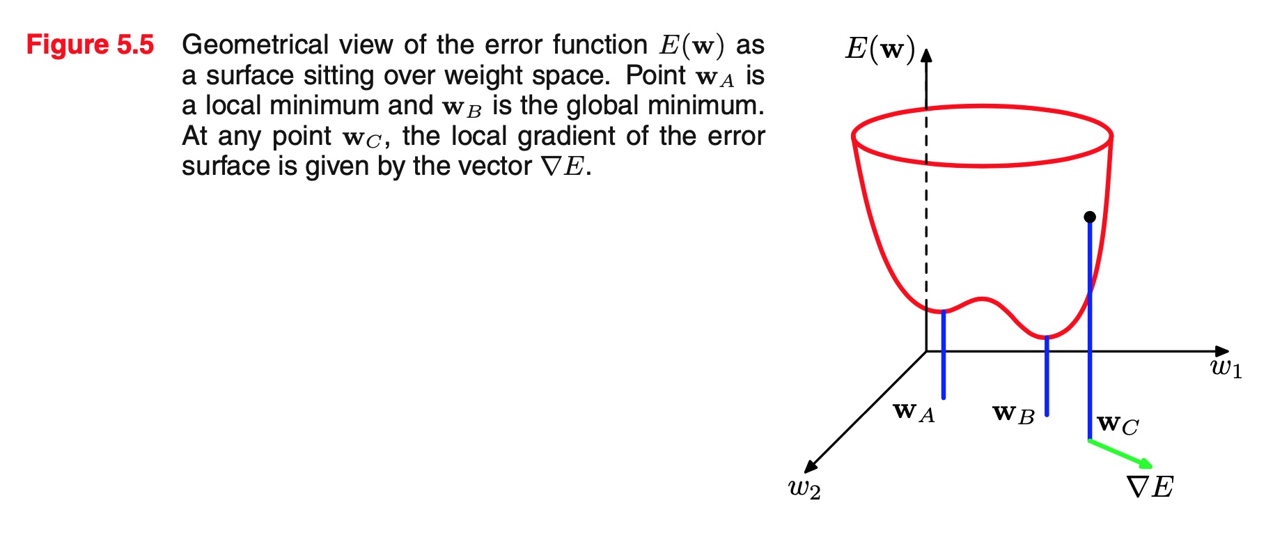
First note that if we make a small step in weight space from $\bold w$ to $\bold w+ \delta\bold w$ then the change in the error function is $\delta E \simeq \delta \bold w^T\nabla E(\bold w)$, where the vector $\nabla E(\bold w)$ points in the direction of greatest rate of increase of the error function. Because the error $E(\bold w)$ is a smooth continuous function of $\bold w$, its smallest value will occur at a point in weight space such that the gradient of the error function vanishes, so that

$\nabla E(\bold w) = 0$

as otherwise we could make a small step in the direction of $-\nabla E(\bold w)$ and thereby further reduce the error. Points at which the gradient vanishes are called stationary points, and may be further classified into minima, maxima, and saddle points.

Our goal is to find a vector w such that $E(\bold w)$ takes its smallest value. However, the error function typically has a highly nonlinear dependence on the weights and bias parameters, and so there will be many points in weight space at which the gradient vanishes (or is numerically very small). Indeed, from the discussion in Section 5.1.1 we see that for any point $\bold w$ that is a local minimum, there will be other points in weight space that are equivalent minima. For instance, in a two-layer network with M hidden units, each point in weight space is a member of a family of $M!2^M$ equivalent points.

Furthermore, there will typically be multiple inequivalent stationary points and in particular multiple inequivalent minima. A minimum that corresponds to the smallest value of the error function for any weight vector is said to be a global minimum. Any other minima corresponding to higher values of the error function are said to be local minima. For a successful application of neural networks, it may not be necessary to find the global minimum (and in general it will not be known whether the global minimum has been found) but it may be necessary to compare several local minima in order to find a sufficiently good solution.

Because there is clearly no hope of finding an analytical solution to the equation $\nabla E(\bold w) = 0$ we resort to iterative numerical procedures. The optimization of continuous nonlinear functions is a widely studied problem and there exists an extensive literature on how to solve it efficiently. Most techniques involve choosing some initial value $\bold w^{(0)}$ for the weight vector and then moving through weight space in a succession of steps of the form

$\bold w^{(\tau +1)} = \bold w^{(\tau)} + \Delta\bold w^{(\tau)} \tag{5.2.2.0}$

Different algorithms involve different choices for the weight vector update $\Delta\bold w^{(\tau)}$.
Many algorithms make use of gradient information and therefore require that, after each update, the value of $\nabla E(\bold w)$ is evaluated at the new weight $\bold w^{(\tau +1)}$
. In order to understand the importance of gradient information, it is useful to consider a local approximation to the error function based on a Taylor expansion.

Local quadratic approximation

Insight into the optimization problem, and into the various techniques for solving it, can be obtained by considering a local quadratic approximation to the error function.

Consider the Taylor expansion of $E(\bold w)$ around some point $\hat \bold w$ in weight space

$E(\bold w) \simeq E(\hat \bold w) + (\bold w - \hat \bold w)^T\bold b + \frac{1}{2} (\bold w - \hat \bold w)^TH (\bold w - \hat \bold w) \tag{5.2.2}$

where cubic and higher terms have been omitted. Here $\bold b$ is defined to be the gradient of $E$ evaluated at $\hat \bold w$

$\bold b \equiv \nabla E|_{\bold w = \hat\bold w} \tag{5.2.3}$

and the Hessian matrix $H = \nabla \nabla E$ has elements

$(H)_{ij} \equiv \frac{\partial E}{\partial w_i \partial w_j}|_{\bold w = \hat\bold w} \tag{5.2.4}$

From (5.2.2), the corresponding local approximation to the gradient is given by

$\nabla E \simeq \bold b + H(\bold w - \hat \bold w) \tag{5.2.4}$

For points $\bold w$ that are sufficiently close to $\hat \bold w$, these expressions will give reasonable approximations for the error and its gradient.

Consider the particular case of a local quadratic approximation around a point $\bold w*$ that is a minimum of the error function. In this case there is no linear term. As $\nabla E = 0$ at $\bold w^*$ , and (5.2.2) becomes

$E(\bold w) = E(\bold w*) + \frac{1}{2} (\bold w - \bold w^*)^TH (\bold w - \bold w^*) \tag{5.2.5}$

where the Hessian H is evaluated at $\bold w^*$ . In order to interpret this geometrically, consider the eigenvalue equation for the Hessian matrix

$H\bold u_i = λ_i\bold u_i \tag{5.2.6}$

where the eigenvectors $u_i$ form a complete orthonormal set so that $\bold u_i^T \bold u_j =\delta_{ij}$.
We now expand $(\bold w - \bold w^*)$ as a linear combination of the eigenvectors in the form

$\bold w - \bold w^* = \sum_ia_i\bold u_i \tag{5.2.7}$

This can be regarded as a transformation of the coordinate system in which the origin is translated to the point $\bold w^*$ , and the axes are rotated to align with the eigenvectors. Then the error function to be written in the form

$E(\bold w) = E(\bold w^*) + \frac{1}{2}\sum_i\lambda_ia_i^2 \tag{5.2.8}$

A matrix H is said to be positive definite if, and only if

$\bold v^TH\bold v \gt 0 \hspace{1em} \text{for all }\bold v \tag{5.2.9}$

Because the eigenvectors $\{\bold u_i\}$ form a complete set, an arbitrary vector $\bold v$ can be written in the form

$\bold v = \sum_ic_i\bold u_i \tag{5.2.10}$

then we have

$\bold v^TH\bold v = \sum_ic_i^2\lambda_i \tag{5.210}$

and so H will be positive definite if, and only if, all of its eigenvalues are positive. In the new coordinate system, whose basis vectors are given by the eigenvectors $\{\bold u_i\}$, the contours of constant E are ellipses centred on the origin, as illustrated in follow. For a one-dimensional weight space, a stationary point w will be a minimum if

$\frac{\partial ^2 E}{\partial w^2}|_{w^*} \gt 0 \tag{5.2.11}$

The corresponding result in D-dimensions is that the Hessian matrix, evaluated at $\bold w^*$ , should be positive definite.

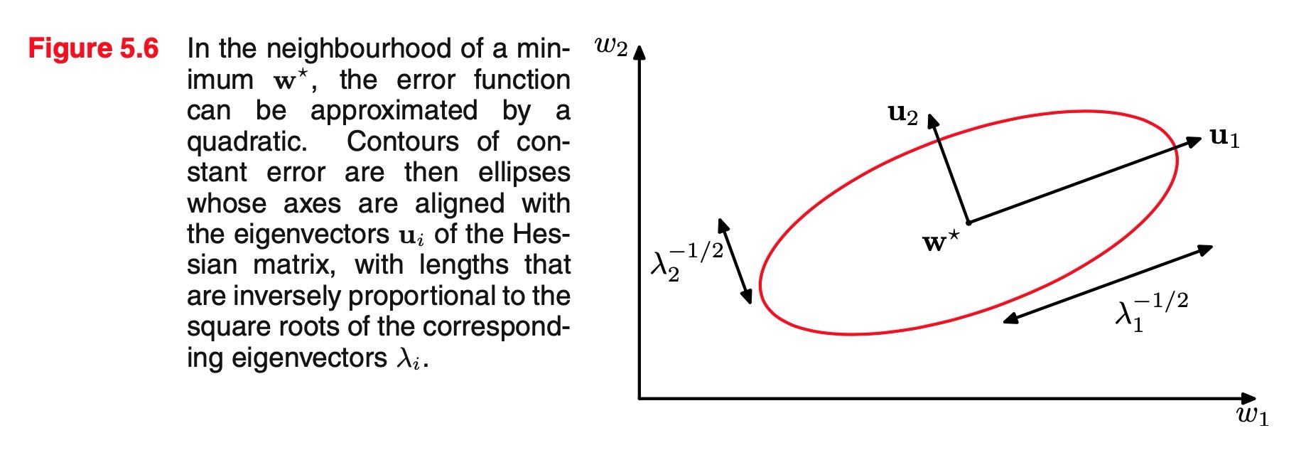
Use of gradient information

As we shall see in Section 5.3, it is possible to evaluate the gradient of an error function efficiently by means of the backpropagation procedure. The use of this gradient information can lead to significant improvements in the speed with which the minima of the error function can be located. We can see why this is so, as follows.

In the quadratic approximation to the error function the error surface is specified by the quantities b and H, which contain a total of $W(W + 3)/2$ independent elements (because the matrix H is symmetric), where $W$ is the dimensionality of $\bold w$ (i.e., the total number of adaptive parameters in the network). The location of the minimum of this quadratic approximation therefore depends on $O(W^2)$ parameters, and we should not expect to be able to locate the minimum until we have gathered $O(W^2)$ independent pieces of information. If we do not make use of gradient information, we would expect to have to perform $O(W^2)$ function evaluations, each of which would require $O(W)$ steps. Thus, the computational effort needed to find the minimum using such an approach would be $O(W^3)$.

Now compare this with an algorithm that makes use of the gradient information. Because each evaluation of $\nabla E$ brings $W$ items of information, we might hope to find the minimum of the function in $O(W)$ gradient evaluations. As we shall see, by using error backpropagation, each such evaluation takes only $O(W)$ steps and so the minimum can now be found in $O(W^2)$ steps. For this reason, the use of gradient information forms the basis of practical algorithms for training neural networks.

Gradient descent optimization

The simplest approach to using gradient information is to choose the weight update in (5.2.2.0) to comprise a small step in the direction of the negative gradient, so that

$\bold w^{(\tau +1)} = \bold w^{(\tau)} - \eta \nabla E(\bold w^{(\tau)}) \tag{5.2.2.0}$

where the parameter $\eta \gt 0$ is known as the learning rate.
After each such update, the gradient is re-evaluated for the new weight vector and the process repeated.

Note that the error function is defined with respect to a training set, and so each step requires that the entire training set be processed in order to evaluate $\nabla E$.Techniques that use the whole data set at once are called batch methods. At each step the weight vector is moved in the direction of the greatest rate of decrease of the error function, and so this approach is known as gradient descent or steepest descent. Although such an approach might intuitively seem reasonable, in fact it turns out to be a poor algorithm, for reasons discussed in Bishop and Nabney (2008).

Error Backpropagation

Our goal in this section is to find an efficient technique for evaluating the gradient of an error function $E(\bold w)$ for a feed-forward neural network. We shall see that this can be achieved using a local message passing scheme in which information is sent alternately forwards and backwards through the network and is known as error backpropagation, or sometimes simply as backprop.

Evaluation of error-function derivatives

We now derive the backpropagation algorithm for a general network having ar- bitrary feed-forward topology, arbitrary differentiable nonlinear activation functions, and a broad class of error function. The resulting formulae will then be illustrated using a simple layered network structure having a single layer of sigmoidal hidden units together with a sum-of-squares error.

Many error functions of practical interest, for instance those defined by maxi- mum likelihood for a set of i.i.d. data, comprise a sum of terms, one for each data point in the training set, so that

$E(\bold w) = \sum_{n=1}^NE_n(\bold w) \tag{5.3.1}$

Here we shall consider the problem of evaluating $\nabla E_n(\bold w)$ for one such term in the error function. This may be used directly for sequential optimization, or the results can be accumulated over the training set in the case of batch methods.

Consider first a simple linear model in which the outputs $y_k$ are linear combinations of the input variables $x_i$ so that

$y_k = \sum_iw_{ki}x_i \tag{5.3.2}$

together with an error function that, for a particular input pattern n, takes the form

$E_n = \frac{1}{2}\sum_k(y_{nk} - t_{nk})^2 \tag{5.3.3}$

where $y_{nk} = y_k (\bold x_n , \bold w)$, The gradient of this error function with respect to a weight $w_{ji}$ is given by

$\frac{\partial E_n}{\partial w_{ji}} = (y_{nj} - t_{nj})x_{ni} \tag{5.3.4}$

which can be interpreted as a ‘local’ computation involving the product of an ‘error signal’ $y_{nj} - t_{nj}$ associated with the output end of the link $w_{ji}$ and the variable xni associated with the input end of the link. In Section 4.3.2, we saw how a similar formula arises with the logistic sigmoid activation function together with the cross entropy error function, and similarly for the softmax activation function together with its matching cross-entropy error function.We shall now see how this simple result extends to the more complex setting of multilayer feed-forward networks.

In a general feed-forward network, each unit computes a weighted sum of its inputs of the form

$a_j = \sum_iw_{ji}z_i \tag{5.3.5}$

where $z_i$ is the activation of a unit, or input, that sends a connection to unit $j$, and $w_{ji}$ is the weight associated with that connection.In Section 5.1, we saw that biases can be included in this sum by introducing an extra unit, or input, with activation fixed at +1.We therefore do not need to deal with biases explicitly. The sum in (5.3.5) is transformed by a nonlinear activation function $h(·)$ to give the activation $z_j$ of unit $j$ in the form

$z_j = h(a_j) \tag{5.3.6}$

Note that one or more of the variables $z_i$ in the sum in (5.3.5) could be an input, and similarly, the unit $j$ in (5.3.6) could be an output.

For each pattern in the training set, we shall suppose that we have supplied the corresponding input vector to the network and calculated the activations of all of the hidden and output units in the network by successive application of (5.3.5) and (5.3.6). This process is often called forward propagation because it can be regarded as a forward flow of information through the network.

Now consider the evaluation of the derivative of $E_n$ with respect to a weight $w_{ji}$. The outputs of the various units will depend on the particular input pattern n. However, in order to keep the notation uncluttered, we shall omit the subscript n from the network variables. First we note that $E_n$ depends on the weight $w_{ji}$ only via the summed input $a_j$ to unit $j$. We can therefore apply the chain rule for partial derivatives to give

$\frac{\partial E_n}{\partial w_{ji}} = \frac{\partial E_n}{\partial a_{j}} \frac{\partial a_j}{\partial w_{ji}} \tag{5.3.7}$

We now introduce a useful notation

$\delta_j \equiv \frac{\partial E_n}{\partial a_j} \tag{5.3.8}$

where the $\delta$ are often referred to as errors for reasons we shall see shortly. (5.3.5), we can write

$\frac{\partial a_j}{\partial w_{ji}} = z_i \tag{5.3.9}$

with above, we then obtain

$\frac{\partial E_n}{\partial w_{ji}} =\delta_jz_i \tag{5.3.10}$

Equation (5.3.10) tells us that the required derivative is obtained simply by multiplying the value of $\delta$ for the unit at the output end of the weight by the value of z for the unit at the input end of the weight (where z = 1 in the case of a bias). Note that this takes the same form as for the simple linear model considered at the start of this section. Thus, in order to evaluate the derivatives, we need only to calculate the value of δj for each hidden and output unit in the network, and then apply (5.3.10).

As we have seen already, for the output units, we have

$\delta_k = y_k - t_k \tag{5.3.11}$

provided we are using the canonical link as the output-unit activation function. To evaluate the $\delta$ for hidden units, we again make use of the chain rule for partial derivatives

$\delta_j \equiv \frac{\partial E_n}{\partial a_j} = \sum_k\frac{\partial E_n}{\partial a_k} \frac{\partial a_k}{\partial a_j} \tag{5.3.12}$

where the sum runs over all units $k$ to which unit $j$ sends connections. The arrangement of units and weights is illustrated as follow.

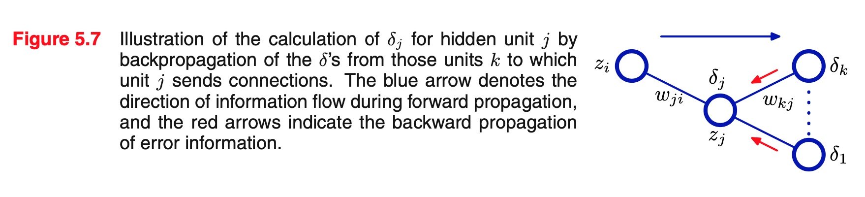
Note that the units labelled k could include other hidden units and/or output units. In writing down (5.3.12), we are making use of the fact that variations in $a_j$ give rise to variations in the error function only through variations in the variables $a_k$.

backpropagation formula

If we now substitute the definition of $\delta$ given by (5.3.8) into (5.3.12), and make use of (5.3.5) and (5.3.6), we obtain the following backpropagation formula

$\delta_j = h'(a_j)\sum_kw_{kj}\delta_k \tag{5.3.13}$

which tells us that the value of $\delta$ for a particular hidden unit can be obtained by propagating the $\delta$ backwards from units higher up in the network

Note that the summation in (5.3.13) is taken over the first index on $w_{kj}$ (corresponding to backward propagation of information through the network), whereas in the forward propagation equation (5.1.9) it is taken over the second index. Because we already know the values of the $\delta$ for the output units, it follows that by recursively applying (5.3.13) we can evaluate the $\delta$ for all of the hidden units in a feed-forward network, regardless of its topology.

Error Backpropagation
The backpropagation procedure can therefore be summarized as follows.

1: Apply an input vector $\bold x_n$ to the network and forward propagate through the network using (5.3.5) and (5.3.6) to find the activations of all the hidden and output units.
2: Evaluate the $\delta_k$ for all the output units using (5.3.11).
3: Backpropagate the $\delta$ using (5.3.13) to obtain $\delta_j$ for each hidden unit in the
network.
4: Use (5.3.10) to evaluate the required derivatives.

For batch methods, the derivative of the total error E can then be obtained by repeating the above steps for each pattern in the training set and then summing over all patterns:

$\frac{\partial E}{\partial w_{ji}} = \sum_n\frac{\partial E_n}{\partial w_{ji}} \tag{5.3.14}$

In the above derivation we have implicitly assumed that each hidden or output unit in the network has the same activation function $h(·)$. The derivation is easily generalized, however, to allow different units to have individual activation functions, simply by keeping track of which form of $h(·)$ goes with which unit.

A simple example

[Skip]

Efficiency of backpropagation

ne of the most important aspects of backpropagation is its computational effi- ciency. To understand this, let us examine how the number of computer operations required to evaluate the derivatives of the error function scales with the total number $W$ of weights and biases in the network.A single evaluation of the error function (for a given input pattern) would require $O(W)$ operations,for sufficiently large $W$ . This follows from the fact that, except for a network with very sparse connections, the number of weights is typically much greater than the number of units, and so the bulk of the computational effort in forward propagation is concerned with evaluat- ing the sums in (5.3.5), with the evaluation of the activation functions representing a small overhead. Each term in the sum in (5.3.5) requires one multiplication and one addition, leading to an overall computational cost that is $O(W)$.

An alternative approach to backpropagation for computing the derivatives of the error function is to use finite differences. This can be done by perturbing each weight in turn, and approximating the derivatives by the expression

$\frac{\partial E_n}{\partial w_{ji}} = \frac{E_n(w_{ji} + \varepsilon) - E_n(w_{ji})}{\varepsilon } + O(\varepsilon), \varepsilon \ll 1 \tag{5.3.15}$

In a software simulation, the accuracy of the approximation to the derivatives can be improved by making $\varepsilon$ smaller, until numerical roundoff problems arise. The accuracy of the finite differences method can be improved significantly by using symmetrical central differences of the form

$\frac{\partial E_n}{\partial w_{ji}} = \frac{E_n(w_{ji} + \varepsilon) - E_n(w_{ji} - \varepsilon)}{2\varepsilon} + O(\varepsilon^2), \varepsilon \ll 1 \tag{5.3.16}$

In this case, the $O(\varepsilon)$ corrections cancel, as can be verified by Taylor expansion on the right-hand side of (5.3.16), and so the residual corrections are $O(\varepsilon^2)$. The number of computational steps is, however, roughly doubled compared with (5.3.15).

The main problem with numerical differentiation is that the highly desirable $O(W)$ scaling has been lost.Each forward propagation requires $O(W)$ steps, and there are $W$ weights in the network each of which must be perturbed individually, so that the overall scaling is $O(W^2)$.

However, numerical differentiation plays an important role in practice, because a comparison of the derivatives calculated by backpropagation with those obtained using central differences provides a powerful check on the correctness of any software implementation of the backpropagation algorithm. When training networks in prac- tice, derivatives should be evaluated using backpropagation, because this gives the greatest accuracy and numerical efficiency. However, the results should be compared with numerical differentiation using (5.3.16) for some test cases in order to check the correctness of the implementation.

The Jacobian matrix

We have seen how the derivatives of an error function with respect to the weights can be obtained by the propagation of errors backwards through the network. The technique of backpropagation can also be applied to the calculation of other deriva- tives. Here we consider the evaluation of the Jacobian matrix, whose elements are given by the derivatives of the network outputs with respect to the inputs

$J_{ki} \equiv \frac{\partial y_k}{\partial x_i} \tag{5.3.17}$

where each such derivative is evaluated with all other inputs held fixed. Jacobian matrices play a useful role in systems built from a number of distinct modules, as illustrated follow.

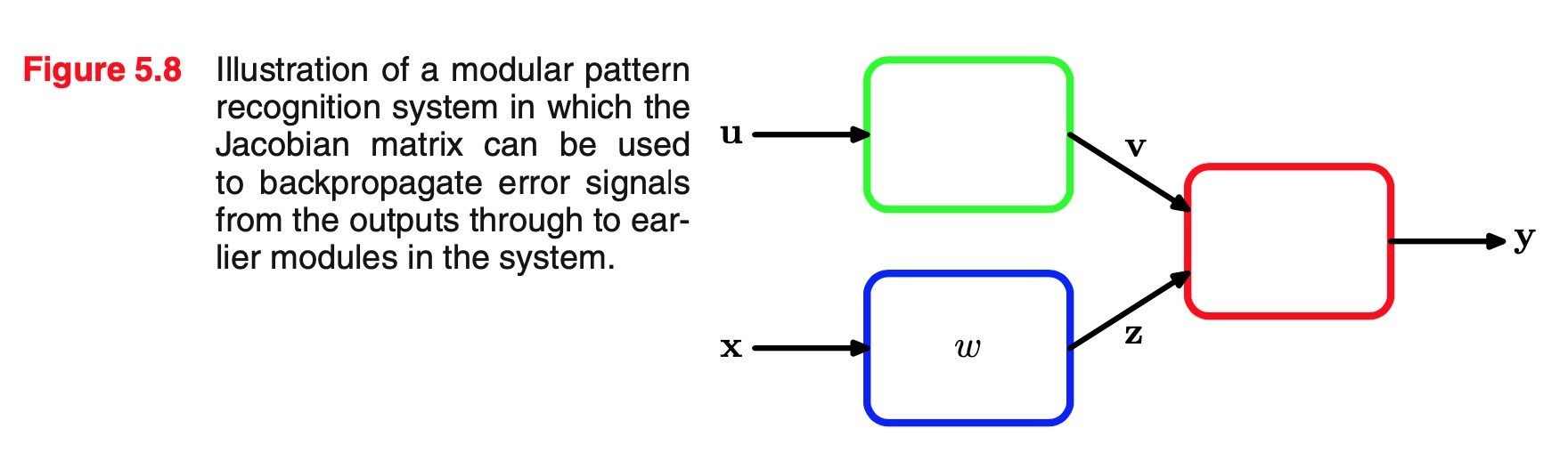
Each module can comprise a fixed or adaptive function, which can be linear or nonlinear, so long as it is differentiable. Suppose we wish to minimize an error function $E$ with respect to the parameter $\bold w$. The derivative of the error function is given by

$\frac{\partial E}{\partial w} = \sum_{k,j}\frac{\partial E}{\partial y_k}\frac{\partial y_k}{\partial z_j}\frac{\partial z_j}{\partial w}\tag{5.3.18}$

in which the Jacobian matrix for the red module in Figure appears in the middle term.

Because the Jacobian matrix provides a measure of the local sensitivity of the outputs to changes in each of the input variables, it also allows any known errors $\Delta x_i$ associated with the inputs to be propagated through the trained network in order to estimate their contribution $\Delta y_k$ to the errors at the outputs, through the relation

$\Delta y_k \simeq \sum_i\frac{\partial y_k}{\partial x_i}\Delta x_i \tag{5.3.19}$

which is valid provided the $|\Delta x_i|$ are small.

In general, the network mapping represented by a trained neural network will be nonlinear, and so the elements of the Jacobian matrix will not be constants but will depend on the particular input vector used. Thus (5.3.19) is valid only for small perturbations of the inputs, and the Jacobian itself must be re-evaluated for each new input vector.

The Jacobian matrix can be evaluated using a backpropagation procedure that is similar to the one derived earlier for evaluating the derivatives of an error function with respect to the weights. We start by writing the element Jki in the form

$J_{ki} = \frac{\partial y_k}{\partial x_i} = \sum_j\frac{\partial y_k}{\partial a_j}\frac{\partial a_j}{\partial x_i} = \sum_jw_{ji}\frac{\partial y_k}{\partial a_j} \tag{5.3.20}$

where we have made use of (5.3.5). The sum in (5.3.20) runs over all units j to which the input unit i sends connections (for example, over all units in the first hidden layer in the layered topology considered earlier).

We now write down a recursive backpropagation formula to determine the derivatives $\partial y_k/\partial a_j$

$\frac{\partial y_k}{\partial a_j} = \sum_l \frac{\partial y_k}{\partial a_l} \frac{\partial a_l}{\partial a_j} = h'(a_j)\sum_lw_{lj}\frac{\partial y_k}{\partial a_l}\tag{5.3.21}$

where the sum runs over all units $l$ to which unit $j$ sends connections (corresponding to the first index of $w_{lj}$).Again, we have made use of (5.3.5) and (5.3.6). This backpropagation starts at the output units for which the required derivatives can be found directly from the functional form of the output-unit activation function. For instance, if we have individual sigmoidal activation functions at each output unit, then

$\frac{\partial y_k}{\partial a_j} = \delta_{kj}\sigma'(a_j) \tag{5.3.22}$

whereas for softmax outputs we have

$\frac{\partial y_k}{\partial a_j} = \delta_{kj}y_k - y_ky_j \tag{5.3.23}$

We can summarize the procedure for evaluating the Jacobian matrix as follows. Apply the input vector corresponding to the point in input space at which the Jacobian matrix is to be found, and forward propagate in the usual way to obtain the activations of all of the hidden and output units in the network. Next, for each row k of the Jacobian matrix, corresponding to the output unit $k$, backpropagate using the recursive relation (5.3.21), starting with (5.3.22) or (5.3.23), for all of the hidden units in the network.Finally, use (5.3.23) to do the backpropagation to the inputs. The Jacobian can also be evaluated using an alternative forward propagation formalism, which can be derived in an analogous way to the backpropagation approach given here.

Again, the implementation of such algorithms can be checked by using numeri- cal differentiation in the form

$\frac{\partial y_k}{\partial x_i} = \frac{y_k(x_i + \varepsilon) - y_k(x_i - \varepsilon)}{2\varepsilon} + O(\varepsilon^2), \varepsilon \ll 1 \tag{5.3.24}$

which involves 2D forward propagations for a network having D inputs.

The Hessian Matrix

We have shown how the technique of backpropagation can be used to obtain the first derivatives of an error function with respect to the weights in the network. Back- propagation can also be used to evaluate the second derivatives of the error, given by

$\frac{\partial ^2E}{\partial w_{ji} \partial w_{lk}}\tag{5.4.1}$

Note that it is sometimes convenient to consider all of the weight and bias parameters as elements $w_i$ of a single vector, denoted $\bold w$, in which case the second derivatives form the elements $H_{ij}$ of the Hessian matrix $H$, where $i,j \in \{1,...,W\}$ and $W$ is the total number of weights and biases. The Hessian plays an important role in many aspects of neural computing, including the following:

1. Several nonlinear optimization algorithms used for training neural networks are based on considerations of the second-order properties of the error surface, which are controlled by the Hessian matrix
2. The Hessian forms the basis of a fast procedure for re-training a feed-forward network following a small change in the training data
3. The inverse of the Hessian has been used to identify the least significant weights in a network as part of network pruning algorithms
4. The Hessian plays a central role in the Laplace approximation for a Bayesian neural network.Its inverse is used to determine the predic- tive distribution for a trained network, its eigenvalues determine the values of hyperparameters, and its determinant is used to evaluate the model evidence.

Various approximation schemes have been used to evaluate the Hessian matrix for a neural network. However, the Hessian can also be calculated exactly using an extension of the backpropagation technique.

An important consideration for many applications of the Hessian is the efficiency with which it can be evaluated. If there are $W$ parameters (weights and biases) in the network, then the Hessian matrix has dimensions $W \times W$ and so the computational effort needed to evaluate the Hessian will scale like $O(W^2)$ for each pattern in the data set. As we shall see, there are efficient methods for evaluating the Hessian whose scaling is indeed $O(W^2)$.

Diagonal approximation

Some of the applications for the Hessian matrix discussed above require the inverse of the Hessian, rather than the Hessian itself. For this reason, there has been some interest in using a diagonal approximation to the Hessian, in other words one that simply replaces the off-diagonal elements with zeros, because its inverse is trivial to evaluate. Again, we shall consider an error function that consists of a sum of terms, one for each pattern in the data set, so that $E = \sum_nE_n$. The Hessian can then be obtained by considering one pattern at a time, and then summing the results over all patterns. From (5.3.5), the diagonal elements of the Hessian, for pattern n, can be written

$\frac{\partial ^2E_n}{\partial w_{ji}^2} = \frac{\partial ^2E_n}{\partial a_j^2}z_i^2\tag{5.4.2}$

Using (5.3.5) and (5.3.6), the second derivatives on the right-hand side of (5.4.2) can be found recursively using the chain rule of differential calculus to give a backprop- agation equation of the form

$\frac{\partial ^2E_n}{\partial a_j^2} = h'(a_j)^2\sum_k\sum_{k'}w_{kj}w_{k'j} \frac{\partial ^2E_n}{\partial a_k \partial a_{k'}} +h''(a_j)\sum_kw_{kj}\frac{\partial E^n}{\partial a_k} \tag{5.4.3}$

If we now neglect off-diagonal elements in the second-derivative terms, we obtain

$\frac{\partial ^2E_n}{\partial a_j^2} = h'(a_j)^2\sum_k w_{kj}^2\frac{\partial ^2E_n}{\partial^2 a_k} +h''(a_j)\sum_kw_{kj}\frac{\partial E^n}{\partial a_k} \tag{5.4.4}$

Note that the number of computational steps required to evaluate this approximation is $O(W)$, where $W$ is the total number of weight and bias parameters in the network, compared with $O(W^2)$ for the full Hessian.

Ricotti et al. (1988) also used the diagonal approximation to the Hessian, but they retained all terms in the evaluation of $\partial^2E_n/\partial a_j^2$ and so obtained exact expres- sions for the diagonal terms. Note that this no longer has $O(W)$ scaling. The major problem with diagonal approximations, however, is that in practice the Hessian is typically found to be strongly nondiagonal, and so these approximations, which are driven mainly be computational convenience, must be treated with care.

Outer product approximation

When neural networks are applied to regression problems, it is common to use a sum-of-squares error function of the form

$E = \frac{1}{2}\sum_{n=1}^{N}(y_n - t_n)^2 \tag{5.4.5}$

where we have considered the case of a single output in order to keep the notation simple (the extension to several outputs is straightforward). We can then write the Hessian matrix in the form

$H = \nabla \nabla E = \sum_{n=1}^N \nabla y_n\nabla y_n + \sum_{n=1}^{N}(y_n - t_n)\nabla\nabla y_n \tag{5.4.6}$

If the network has been trained on the data set, and its outputs $y_n$ happen to be very close to the target values tn, then the second term in (5.4.6) will be small and can be neglected. More generally, however, it may be appropriate to neglect this term by the following argument.Recall from Section 1.6.5 that the optimal function that minimizes a sum-of-squares loss is the conditional average of the target data. The quantity $(y_n − t_n)$ is then a random variable with zero mean. If we assume that its value is uncorrelated with the value of the second derivative term on the right-hand side of (5.4.6), then the whole term will average to zero in the summation over $n$.

By neglecting the second term in (5.4.6), we arrive at the Levenberg–Marquardt approximation or outer product approximation (because the Hessian matrix is built up from a sum of outer products of vectors), given by

$H \simeq \sum_{n=1}^N\bold b_n\bold b_n^T \tag{5.4.7}$

where $b_n = \nabla y_n =\nabla a_n$ because the activation function for the output units is simply the identity. Evaluation of the outer product approximation for the Hessian is straightforward as it only involves first derivatives of the error function, which can be evaluated efficiently in $O(W)$ steps using standard backpropagation. The elements of the matrix can then be found in $O(W^2)$ steps by simple multiplication. It is important to emphasize that this approximation is only likely to be valid for a network that has been trained appropriately, and that for a general network mapping the second derivative terms on the right-hand side of (5.4.6) will typically not be negligible.

In the case of the cross-entropy error function for a network with logistic sigmoid output-unit activation functions, the corresponding approximation is given by

$H \simeq \sum_{n=1}^N y_n(1-y_n)\bold b_n\bold b_n^T \tag{5.4.8}$

An analogous result can be obtained for multiclass networks having softmax output-unit activation functions.

Inverse Hessian

We can use the outer-product approximation to develop a computationally ef- ficient procedure for approximating the inverse of the Hessian (Hassibi and Stork, 1993). First we write the outer-product approximation in matrix notation as

$H_N = \sum_{n=1}^N \bold b_n\bold b_n^T \tag{5.4.9}$

where $\bold b_n \equiv \nabla_{\bold w} a_n$ is the contribution to the gradient of the output unit activation arising from data point $n$. We now derive a sequential procedure for building up the Hessian by including data points one at a time. Suppose we have already obtained the inverse Hessian using the first $L$ data points. By separating off the contribution from data point $L + 1$, we obtain

$H_{L + 1} = H_L + \bold b_{L+1}\bold b_{L+1}^T \tag{5.4.10}$

In order to evaluate the inverse of the Hessian, we now consider the matrix identity

$(M + \bold v\bold v^T)^{-1} = M^{-1} - \frac{(M^{-1}\bold v)(\bold v^TM^{-1})}{1 + \bold v^TM^{-1}\bold v} \tag{5.4.11}$

where $I$ is the unit matrix, which is simply a special case of the Woodbury identity(C.7). If we now identify $H_L$ with $M$ and $\bold b_{L+1}$ with $\bold v$, we obtain

$H_{L+1}^{-1} = H_L^{-1} - \frac{H_L^{-1}\bold b_{L+1}\bold b_{L+1}^TH_L^{-1}}{1 + \bold b_{L+1}^TH_L^{-1}\bold b_{L+1}} \tag{5.4.12}$

In this way, data points are sequentially absorbed until $L+1 = N$ and the whole data set has been processed. This result therefore represents a procedure for evaluating the inverse of the Hessian using a single pass through the data set. The initial matrix $H_0$ is chosen to be $\alpha I$, where α is a small quantity, so that the algorithm actually finds the inverse of $H + \alpha I$. The results are not particularly sensitive to the precise value of $\alpha$. Extension of this algorithm to networks having more than one output is straightforward.

We note here that the Hessian matrix can sometimes be calculated indirectly as part of the network training algorithm. In particular, quasi-Newton nonlinear opti- mization algorithms gradually build up an approximation to the inverse of the Hes- sian during training. Such algorithms are discussed in detail in Bishop and Nabney (2008).

Finite differences

As in the case of the first derivatives of the error function, we can find the second derivatives by using finite differences, with accuracy limited by numerical precision. If we perturb each possible pair of weights in turn, we obtain

$\frac{\partial ^2E}{\partial w_{ji}\partial w_{lk}} = \frac{1}{4\varepsilon} \{E(w_{ji} + \varepsilon, w_{lk} + \varepsilon) - E(w_{ji} + \varepsilon, w_{lk} - \varepsilon) \\ - E(w_{ji} - \varepsilon, w_{lk} + \varepsilon) + E(w_{ji} - \varepsilon, w_{lk} - \varepsilon) \} + O(\varepsilon^2)\tag{5.4.13}$

Again, by using a symmetrical central differences formulation, we ensure that the residual errors are $O(\varepsilon^2)$ rather than $O(\varepsilon)$. Because there are $W^2$ elements in the Hessian matrix, and because the evaluation of each element requires four forward propagations each needing $O(W)$ operations (per pattern), we see that this approach will require $O(W^3)$ operations to evaluate the complete Hessian. It therefore has poor scaling properties, although in practice it is very useful as a check on the software implementation of backpropagation methods.

A more efficient version of numerical differentiation can be found by applying central differences to the first derivatives of the error function, which are themselves calculated using backpropagation. This gives

$\frac{\partial ^2E}{\partial w_{ji}\partial w_{lk}} = \frac{1}{2\varepsilon} \{\frac{\partial E}{\partial w_{ji}}(w_{lk} + \varepsilon) - \frac{\partial E}{\partial w_{ji}}(w_{lk} - \varepsilon)\} + O(\varepsilon^2)\tag{5.4.14}$

Because there are now only $W$ weights to be perturbed, and because the gradients can be evaluated in $O(W)$ steps, we see that this method gives the Hessian in $O(W^2)$ operations.

Exact evaluation of the Hessian

So far, we have considered various approximation schemes for evaluating the Hessian matrix or its inverse. The Hessian can also be evaluated exactly, for a net- work of arbitrary feed-forward topology, using extension of the technique of back- propagation used to evaluate first derivatives, which shares many of its desirable features including computational efficiency (Bishop, 1991; Bishop, 1992). It can be applied to any differentiable error function that can be expressed as a function of the network outputs and to networks having arbitrary differentiable activation func- tions. The number of computational steps needed to evaluate the Hessian scales like $O(W^2)$. Similar algorithms have also been considered by Buntine and Weigend (1993).

Here we consider the specific case of a network having two layers of weights, for which the required equations are easily derived. We shall use indices $i$ and $i'$ to denote inputs, indices $j$ and $j'$ to denoted hidden units, and indices $k$ and $k'$ to denote outputs. We first define

$\delta_k = \frac{\partial E_n}{\partial a_k}, \hspace{3em} M_{kk'} \equiv \frac{\partial ^2E_n}{\partial a_k \partial a_k'} \tag{5.4.15}$

where $E_n$ is the contribution to the error from data point $n$. The Hessian matrix for this network can then be considered in three separate blocks as follows.

• Both weights in the second layer:

$\frac{\partial ^2E_n}{\partial w_{kj}^{(2)} \partial w_{k'j'}^{(2)}} = z_jz_{j'}M_{kk'} \tag{5.4.16}$

• Both weights in the first layer:

$\frac{\partial ^2E_n}{\partial w_{ji}^{(1)} \partial w_{j'i'}^{(1)}} = x_ix_{i'}h''(a_{j'})I_{jj'}\sum_kw_{kj'}^{(2)}\delta_k + x_ix_{i'} h'(a_{j'})h'(a_j)\sum_k\sum_{k'}w_{k'j'}^{(2)}w_{kj}^{(2)} M_{kk'} \tag{5.4.17}$

• One weight in each layer:

$\frac{\partial ^2E_n}{\partial w_{ji}^{(1)} \partial w_{kj'}^{(2)}} = x_ih'(a_{j'})\{ \delta_kI_{jj'} + z_j\sum_{k'} w_{k'j'}^{(2)}H_{kk'}\} \tag{5.4.18}$

Here $I_{jj'}$ is the $j,j'$ element of the identity matrix. If one or both of the weights is a bias term, then the corresponding expressions are obtained simply by setting the appropriate activation(s) to 1. Inclusion of skip-layer connections is straightforward.

Fast multiplication by the Hessian

For many applications of the Hessian, the quantity of interest is not the Hessian matrix $H$ itself but the product of $H$ with some vector $\bold v$. We have seen that the evaluation of the Hessian takes $O(W^2)$ operations, and it also requires storage that is $O(W^2)$. The vector $\bold v^TH$ that we wish to calculate, however, has only $W$ elements, so instead of computing the Hessian as an intermediate step, we can instead try to find an efficient approach to evaluating $\bold v^TH$ directly in a way that requires only $O(W)$ operations.
To do this, we first note that

$\bold v^TH = \bold v^T\nabla(\nabla E) \tag{5.4.19}$

where $\nabla$ denotes the gradient operator in weight space. We can then write down the standard forward-propagation and backpropagation equations for the evaluation of $\nabla E$ and apply (5.4.19) to these equations to give a set of forward-propagation and backpropagation equations for the evaluation of $\bold v^TH$ (Møller, 1993; Pearlmutter, 1994). This corresponds to acting on the original forward-propagation and backpropagation equations with a differential operator $\bold v^T\nabla$. Pearlmutter (1994) used the notation $R{·}$ to denote the operator $\bold v^T\nabla$, and we shall follow this convention.The analysis is straightforward and makes use of the usual rules of differential calculus, together with the result

$R\{\bold w\} = \bold v \tag{5.4.20}$

Regularization in Neural Networks

The number of input and outputs units in a neural network is generally determined by the dimensionality of the data set, whereas the number M of hidden units is a free parameter that can be adjusted to give the best predictive performance. Note that M controls the number of parameters (weights and biases) in the network, and so we might expect that in a maximum likelihood setting there will be an optimum value of M that gives the best generalization performance, corresponding to the optimum balance between under-fitting and over-fitting.

The generalization error, however, is not a simple function of M due to the presence of local minima in the error function.
Here we see the effect of choosing multiple random initializations for the weight vector for a range of values of M. The overall best validation set performance in this case occurred for a particular solution having $M = 8$.

here are, however, other ways to control the complexity of a neural network model in order to avoid over-fitting. From our discussion of polynomial curve fitting in Chapter 1, we see that an alternative approach is to choose a relatively large value for M and then to control complexity by the addition of a regularization term to the error function. The simplest regularizer is the quadratic, giving a regularized error of the form

$\displaystyle \widetilde {E} (\bold w) = E(\bold w) + \frac{\lambda}{2}\bold w^T\bold w \tag{5.5.1}$

This regularizer is also known as weight decay and has been discussed at length in Chapter 3. The effective model complexity is then determined by the choice of the regularization coefficient $\lambda$. As we have seen previously, this regularizer can be interpreted as the negative logarithm of a zero-mean Gaussian prior distribution over the weight vector $\bold w$.

Consistent Gaussian priors

One of the limitations of simple weight decay in the form (5.5.1) is that is inconsistent with certain scaling properties of network mappings.

[TODO]

Early stopping

An alternative to regularization as a way of controlling the effective complexity of a network is the procedure of early stopping. The training of nonlinear network models corresponds to an iterative reduction of the error function defined with re- spect to a set of training data. For many of the optimization algorithms used for network training, such as conjugate gradients, the error is a nonincreasing function of the iteration index. However, the error measured with respect to independent data, generally called a validation set, often shows a decrease at first, followed by an in- crease as the network starts to over-fit. Training can therefore be stopped at the point of smallest error with respect to the validation data set, in order to obtain a network having good generalization performance.

The behaviour of the network in this case is sometimes explained qualitatively in terms of the effective number of degrees of freedom in the network, in which this number starts out small and then to grows during the training process, corresponding to a steady increase in the effective complexity of the model. Halting training before a minimum of the training error has been reached then represents a way of limiting the effective network complexity.

In the case of a quadratic error function, we can verify this insight, and show that early stopping should exhibit similar behaviour to regularization using a sim- ple weight-decay term.

Invariances

In many applications of pattern recognition, it is known that predictions should be unchanged, or invariant, under one or more transformations of the input vari- ables. For example, in the classification of objects in two-dimensional images, such as handwritten digits, a particular object should be assigned the same classification irrespective of its position within the image (translation invariance) or of its size (scale invariance). Such transformations produce significant changes in the raw data, expressed in terms of the intensities at each of the pixels in the image, and yet should give rise to the same output from the classification system. Similarly in speech recognition, small levels of nonlinear warping along the time axis, which preserve temporal ordering, should not change the interpretation of the signal.

If sufficiently large numbers of training patterns are available, then an adaptive model such as a neural network can learn the invariance, at least approximately. This involves including within the training set a sufficiently large number of examples of the effects of the various transformations. Thus, for translation invariance in an im- age, the training set should include examples of objects at many different positions.

This approach may be impractical, however, if the number of training examples is limited, or if there are several invariants (because the number of combinations of transformations grows exponentially with the number of such transformations). We therefore seek alternative approaches for encouraging an adaptive model to exhibit the required invariances. These can broadly be divided into four categories:

1.The training set is augmented using replicas of the training patterns, trans- formed according to the desired invariances. For instance, in our digit recog- nition example, we could make multiple copies of each example in which the digit is shifted to a different position in each image.

2.A regularization term is added to the error function that penalizes changes in the model output when the input is transformed. This leads to the technique of tangent propagation

3.Invariance is built into the pre-processing by extracting features that are invari- ant under the required transformations. Any subsequent regression or classi- fication system that uses such features as inputs will necessarily also respect these invariances.

4.The final option is to build the invariance properties into the structure of a neu- ral network (or into the definition of a kernel function in the case of techniques such as the relevance vector machine). One way to achieve this is through the use of local receptive fields and shared weights, as discussed in the context of convolutional neural networks in Section 5.5.6.

Approach 1 is often relatively easy to implement and can be used to encourage com- plex invariances. For sequential training algorithms, this can be done by transforming each input pattern before it is presented to the model so that, if the patterns are being recycled, a different transformation (drawn from an appropriate distribution) is added each time. For batch methods, a similar effect can be achieved by replicating each data point a number of times and transforming each copy independently. The use of such augmented data can lead to significant improvements in generalization (Simard et al., 2003), although it can also be computationally costly.

Approach 2 leaves the data set unchanged but modifies the error function through the addition of a regularizer. In Section 5.5.5, we shall show that this approach is closely related to approach 2.

One advantage of approach 3 is that it can correctly extrapolate well beyond the range of transformations included in the training set. However, it can be difficult to find hand-crafted features with the required invariances that do not also discard information that can be useful for discrimination.

Tangent propagation

We can use regularization to encourage models to be invariant to transformations of the input through the technique of tangent propagation

Consider the effect of a transformation on a particular input vector $\bold x_n$. Provided the transformation is continuous (such as translation or rotation, but not mirror reflection for instance), then the transformed pattern will sweep out a manifold $\mathcal{M}$ within the D-dimensional input space.

[TODO]

Training with transformed data

We have seen that one way to encourage invariance of a model to a set of transformations is to expand the training set using transformed versions of the original input patterns. Here we show that this approach is closely related to the technique of tangent propagation (Bishop, 1995b; Leen, 1995).

[TODO(With Tangent propagation)]

Convolutional networks

Another approach to creating models that are invariant to certain transformation of the inputs is to build the invariance properties into the structure of a neural net- work. This is the basis for the convolutional neural network (Le Cun et al., 1989; LeCun et al., 1998), which has been widely applied to image data.

Consider the specific task of recognizing handwritten digits. Each input image comprises a set of pixel intensity values, and the desired output is a posterior probability distribution over the ten digit classes. We know that the identity of the digit is invariant under translations and scaling as well as (small) rotations. Furthermore, the network must also exhibit invariance to more subtle transformations such as elastic deformations of the kind as follow. One simple approach would be to treat the image as the input to a fully connected network. Given a sufficiently large training set, such a network could in principle yield a good solution to this problem and would learn the appropriate invariances by example.

However, this approach ignores a key property of images, which is that nearby pixels are more strongly correlated than more distant pixels. Many of the modern approaches to computer vision exploit this property by extracting local features that depend only on small subregions of the image. Information from such features can then be merged in later stages of processing in order to detect higher-order features and ultimately to yield information about the image as whole. Also, local features that are useful in one region of the image are likely to be useful in other regions of the image, for instance if the object of interest is translated.

convolutional_networks

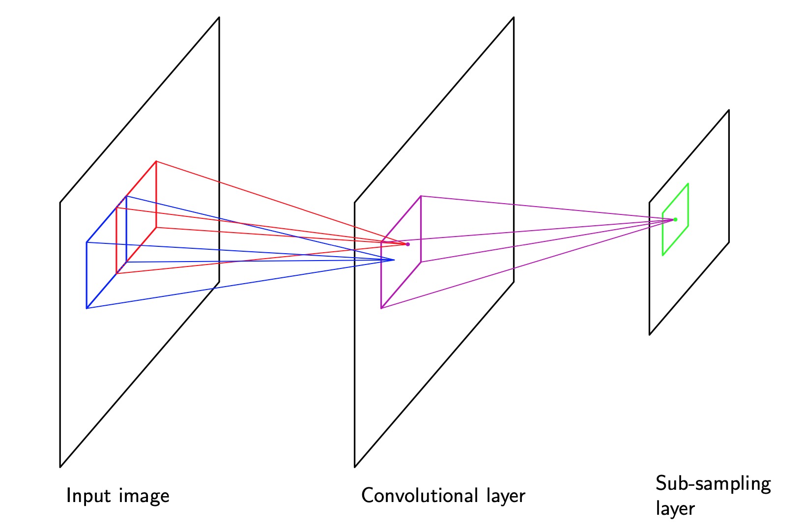
The structure of a convolutional network
These notions are incorporated into convolutional neural networks through three mechanisms:

1. local receptive fields
2. weight sharing
3. subsampling.

In the convolutional layer the units are organized into planes, each of which is called a feature map. Units in a feature map each take inputs only from a small subregion of the image, and all of the units in a feature map are constrained to share the same weight values. For instance, a feature map might consist of 100 units arranged in a 10 × 10 grid, with each unit taking inputs from a 5 × 5 pixel patch of the image. The whole feature map therefore has 25 adjustable weight parameters plus one adjustable bias parameter. Input values from a patch are linearly combined using the weights and the bias, and the result transformed by a sigmoidal nonlinearity using (5.1). If we think of the units as feature detectors, then all of the units in a feature map detect the same pattern but at different locations in the input image. Due to the weight sharing, the evaluation of the activations of these units is equivalent to a convolution of the image pixel intensities with a ‘kernel’ comprising the weight parameters. If the input image is shifted, the activations of the feature map will be shifted by the same amount but will otherwise be unchanged. This provides the basis for the (approximate) invariance of the network outputs to translations and distortions of the input image. Because we will typically need to detect multiple features in order to build an effective model, there will generally be multiple feature maps in the convolutional layer, each having its own set of weight and bias parameters.

The outputs of the convolutional units form the inputs to the subsampling layer of the network. For each feature map in the convolutional layer, there is a plane of units in the subsampling layer and each unit takes inputs from a small receptive field in the corresponding feature map of the convolutional layer. These units perform subsampling. For instance, each subsampling unit might take inputs from a 2 × 2 unit region in the corresponding feature map and would compute the average of those inputs, multiplied by an adaptive weight with the addition of an adaptive bias parameter, and then transformed using a sigmoidal nonlinear activation function. The receptive fields are chosen to be contiguous and nonoverlapping so that there are half the number of rows and columns in the subsampling layer compared with the convolutional layer. In this way, the response of a unit in the subsampling layer will be relatively insensitive to small shifts of the image in the corresponding regions of the input space.

In a practical architecture, there may be several pairs of convolutional and sub- sampling layers. At each stage there is a larger degree of invariance to input trans- formations compared to the previous layer. There may be several feature maps in a given convolutional layer for each plane of units in the previous subsampling layer, so that the gradual reduction in spatial resolution is then compensated by an increas- ing number of features. The final layer of the network would typically be a fully connected, fully adaptive layer, with a softmax output nonlinearity in the case of multiclass classification.

The whole network can be trained by error minimization using backpropagation to evaluate the gradient of the error function. This involves a slight modification of the usual backpropagation algorithm to ensure that the shared-weight constraints are satisfied. Due to the use of local receptive fields, the number of weights in the network is smaller than if the network were fully connected. Furthermore, the number of independent parameters to be learned from the data is much smaller still, due to the substantial numbers of constraints on the weights.

Soft weight sharing

One way to reduce the effective complexity of a network with a large number of weights is to constrain weights within certain groups to be equal. This is the technique of weight sharing that was discussed in Section 5.5.6 as a way of building translation invariance into networks used for image interpretation. It is only appli- cable, however, to particular problems in which the form of the constraints can be specified in advance. Here we consider a form of soft weight sharing (Nowlan and Hinton, 1992) in which the hard constraint of equal weights is replaced by a form of regularization in which groups of weights are encouraged to have similar values. Furthermore, the division of weights into groups, the mean weight value for each group, and the spread of values within the groups are all determined as part of the learning process.

Mixture Density Networks

[Skip]

Bayesian Neural Networks

[Skip]

Kernel Methods

Many linear parametric models can be re-cast into an equivalent ‘dual represen- tation’ in which the predictions are also based on linear combinations of a kernel function evaluated at the training data points. As we shall see, for models which are based on a fixed nonlinear feature space mapping φ(x), the kernel function is given by the relation

$k(\bold x, \bold x') = \phi(\bold x)^T\phi(\bold x') \tag{6.1.1}$

From this definition, we see that the kernel is a symmetric function of its arguments so that $k(\bold x, \bold x') = k(\bold x', \bold x)$.

The kernel concept was introduced into the field of pattern recognition by Aizerman et al. (1964) in the context of the method of potential functions, so-called because of an analogy with electrostatics. Although neglected for many years, it was reintroduced into machine learning in the context of large-margin classifiers by Boser et al. (1992) giving rise to the technique of support vector machines.

The simplest example of a kernel function is obtained by considering the identity mapping for the feature space in (6.1.1) so that $\phi(\bold x) = \bold x$, in which case $k(\bold x, \bold x') = \bold x^T\bold x'$.We shall refer to this as the linear kernel.

Inner Product

The concept of a kernel formulated as an inner product in a feature space allows us to build interesting extensions of many well-known algorithms by making use of the kernel trick, also known as kernel substitution. The general idea is that, if we have an algorithm formulated in such a way that the input vector x enters only in the form of scalar products, then we can replace that scalar product with some other choice of kernel. For instance, the technique of kernel substitution can be applied to principal component analysis in order to develop a nonlinear variant of PCA

Dual Representations

Many linear models for regression and classification can be reformulated in terms of a dual representation in which the kernel function arises naturally. This concept will play an important role when we consider support vector machines in the next chapter.
[TODO]

Constructing Kernels

In order to exploit kernel substitution, we need to be able to construct valid kernel functions. One approach is to choose a feature space mapping $\phi(\bold x)$ and then use this to find the corresponding kernel.
[TODO]

Radial Basis Function Networks

Historically, radial basis functions were introduced for the purpose of exact function interpolation, which have the property that each basis function depends only on the radial distance (typically Euclidean) from a centre $\mu_j$ , so that $\phi_j (\bold x) = h(||\bold x − \mu_j||).$

Given a set of input vectors $\{\bold x_1, . . . ,\bold x_N \}$ along with corresponding target values $\{t_1 , . . . , t_N\}$, the goal is to find a smooth function $f(\bold x)$ that fits every target value exactly, so that $f(\bold x_n) = t_n$ for $n = 1, . . . , N$. This is achieved by expressing $f(\bold x)$ as a linear combination of radial basis functions, one centred on every data point

$f(\bold x) = \sum_{n=1}^Nw_nh(||\bold x - \bold x_n||) \tag{6.1.1}$

The values of the coefficients $\{w_n\}$ are found by least squares, and because there are the same number of coefficients as there are constraints, the result is a function that fits every target value exactly. In pattern recognition applications, however, the target values are generally noisy, and exact interpolation is undesirable because this corresponds to an over-fitted solution.

Gaussian Processes

[TODO]

Sparse Kernel Machines

In the previous chapter, we explored a variety of learning algorithms based on nonlinear kernels. One of the significant limitations of many such algorithms is that the kernel function $k(\bold x_n, \bold x_m)$ must be evaluated for all possible pairs $\bold x_n$ and $\bold x_m$ of training points, which can be computationally infeasible during training and can lead to excessive computation times when making predictions for new data points. In this chapter we shall look at kernel-based algorithms that have sparse solutions, so that predictions for new inputs depend only on the kernel function evaluated at a subset of the training data points.

We begin by looking in some detail at the support vector machine (SVM), which became popular in some years ago for solving problems in classification, regression, and novelty detection.

convex optimization problem

An important property of support vector machines is that the determination of the model parameters corresponds to a convex optimization prob- lem, and so any local solution is also a global optimum.

Maximum Margin Classifiers [Support Vector Machine]

We begin our discussion of support vector machines by returning to the two-class classification problem using linear models of the form

$y(\bold x) = \bold w^T\phi(\bold x) + b \tag{7.1.1}$

where $\phi(\bold x)$ denotes a fixed feature-space transformation, and we have made the bias parameter b explicit.

Note that we shall shortly introduce a dual representation expressed in terms of kernel functions, which avoids having to work explicitly in feature space. The training data set comprises N input vectors $\bold x1, . . . , \bold x_N$ , with corresponding target values $t_1,...,t_N$ where $t_n \in \{−1,1\}$, and new data points $\bold x$ are classified according to the sign of $y(\bold x)$.

We shall assume for the moment that the training data set is linearly separable in feature space, so that by definition there exists at least one choice of the parameters $\bold w$ and $b$ such that a function of the form (7.1.1) satisfies $y(\bold x_n) \gt 0$ for points having $t_n =+1$ and $y(\bold x_n) \lt 0 $ for points having $t_n =−1$,so that

$t_ny(\bold x_n) \gt 0$

for all training data points.

Margin

There may of course exist many such solutions that separate the classes exactly. In Section 4.1.7, we described the perceptron algorithm that is guaranteed to find a solution in a finite number of steps. The solution that it finds, however, will be dependent on the (arbitrary) initial values chosen for $\bold w$ and $b$ as well as on the order in which the data points are presented. If there are multiple solutions all of which classify the training data set exactly, then we should try to find the one that will give the smallest generalization error. The support vector machine approaches this problem through the concept of the margin, which is defined to be the smallest distance between the decision boundary and any of the samples, as illustrated follow.

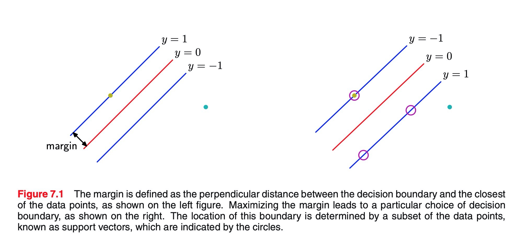
In support vector machines the decision boundary is chosen to be the one for which the margin is maximized. The maximum margin solution can be motivated using computational learning theory, also known as statistical learning theory. However, a simple insight into the origins of maximum margin has been given by Tong and Koller (2000) who consider a framework for classification based on a hybrid of generative and discriminative approaches. They first model the distribution over input vectors $\bold x$ for each class using a Parzen density estimator with Gaussian kernels having a common parameter $\sigma^2$ . Together with the class priors, this defines an optimal misclassification-rate decision boundary. However, instead of using this optimal boundary, they determine the best hyperplane by minimizing the probability of error relative to the learned density model. In the limit $\sigma^2 \to 0$, the optimal hyperplane is shown to be the one having maximum margin. The intuition behind this result is that as $\sigma^2$ is reduced, the hyperplane is increasingly dominated by nearby data points relative to more distant ones. In the limit, the hyperplane becomes independent of data points that are not support vectors.

The perpendicular distance of a point $\bold x$ from a hyper-plane defined by $y(\bold x) = 0$ where $y(\bold x)$ takes the form (7.1.1) is given by $|y(\bold x)|/ \bold w$ . Furthermore, we are only interested in solutions for which all data points are correctly classified, so that $t_ny(\bold x_n) \gt 0$ for all $n$. Thus the distance of a point $\bold x_n$ to the decision surface is given by

$\frac{t_ny(\bold x_n)}{||\bold w||} = \frac{t_n(\bold w^T\phi(\bold x_n) + b)}{||\bold w||} \tag{7.1.2}$

The margin is given by the perpendicular distance to the closest point $\bold x_n$ from the data set, and we wish to optimize the parameters $\bold w$ and $b$ in order to maximize this distance. Thus the maximum margin solution is found by solving

$\argmax_{\bold w, b} \Large \{\normalsize \frac{1}{||\bold w||}\min_n[t_n(\bold w^T\phi(\bold x_n) + b)] \Large \}\normalsize\tag{7.1.3}$

where we have taken the factor $1/ ||\bold w||$ outside the optimization over $n$ because $\bold w$ does not depend on $n$. Direct solution of this optimization problem would be very complex, and so we shall convert it into an equivalent problem that is much easier to solve. To do this we note that if we make the rescaling $\bold w \to k\bold w$ and $b \to kb$, then the distance from any point $\bold x_n$ to the decision surface, given by $t_ny(\bold x_n)/ ||\bold w||$ , is unchanged. We can use this freedom to set

$t_n(\bold w^T\phi(\bold x_n) + b) = 1\tag{7.1.4}$

for the point that is closest to the surface. In this case, all data points will satisfy the constraints

$t_n(\bold w^T\phi(\bold x_n) + b ) \ge 1, \hspace{2em} n = 1,\cdots,N \tag{7.1.5}$

This is known as the canonical representation of the decision hyperplane. In the case of data points for which the equality holds, the constraints are said to be active, whereas for the remainder they are said to be inactive.

By definition, there will always be at least one active constraint, because there will always be a closest point, and once the margin has been maximized there will be at least two active constraints. The optimization problem then simply requires that we maximize $||w||^{−1}$, which is equivalent to minimizing $||w||^2$, and so we have to solve the optimization problem

$\argmin_{\bold w, b} \frac{1}{2}||\bold w||^2 \tag{7.1.6}$

subject to the constraints given by (7.1.5). The factor of 1/2 in (7.1.6) is included for later convenience.

This is an example of a quadratic programming problem in which we are trying to minimize a quadratic function subject to a set of linear inequality constraints. It appears that the bias parameter $b$ has disappeared from the optimization. However, it is determined implicitly via the constraints, because these require that changes to $\bold w$ be compensated by changes to $b$. We shall see how this works shortly.

Lagrange multipliers

In order to solve this constrained optimization problem, we introduce Lagrange multipliers $a_n \ge 0$, with one multiplier $a_n$ for each of the constraints in (7.1.5), giving the Lagrangian function

$L(\bold w, b, \bold a) = \frac{1}{2}||\bold w||^2 - \sum_{n=1}^{N}a_n\{t_n(\bold w^T\phi(\bold x_n) + b) - 1\} \tag{7.1.7}$

where $\bold a = (a_1,\cdots, a_N)^T$. Note the minus sign in front of the Lagrange multiplier term, because we are minimizing with respect to $\bold w$ and $b$, and maximizing with respect to $\bold a$.

Setting the derivatives of $L(\bold w, b, \bold a)$ with respect to $\bold w$ and $b$ equal to zero, we obtain the following two conditions

$\frac{\partial L}{\partial \bold w} = 0 \to \bold w = \sum_{n=1}^Na_nt_n\phi(\bold x_n) \tag{7.1.8}$

$\frac{\partial L}{\partial b} = 0 \to 0 = \sum_{n=1}^Na_nt_n \tag{7.1.9}$

Eliminating $\bold w$ and $b$ from $L(\bold w, b, \bold a)$ using these conditions then gives the dual representation of the maximum margin problem in which we maximize

$\widetilde L(\bold a) = \sum_{n=1}^Na_n - \frac{1}{2}\sum_{n=1}^N\sum_{m=1}^Na_na_mt_nt_mk(\bold x_n, \bold x_m) \tag{7.1.10}$

with respect to $\bold a$ subject to the constraints

$\begin{aligned}\sum_{n=1}^Na_nt_n = 0 \\ a_n \ge 0 \end{aligned} \tag{7.1.11}$

Here the kernel function is defined by $k(\bold x, \bold x') = \phi(\bold x)^T\phi(\bold x')$. Again, this takes the form of a quadratic programming problem in which we optimize a quadratic function of a subject to a set of inequality constraints. We shall discuss techniques for solving such quadratic programming problems next.

The solution to a quadratic programming problem in $M$ variables in general has computational complexity that is $O(M^3)$. In going to the dual formulation we have turned the original optimization problem, which involved minimizing (7.1.6) over $M$ variables, into the dual problem (7.1.10), which has $N$ variables. For a fixed set of basis functions whose number $M$ is smaller than the number $N$ of data points, the move to the dual problem appears disadvantageous. However, it allows the model to be reformulated using kernels, and so the maximum margin classifier can be applied efficiently to feature spaces whose dimensionality exceeds the number of data points, including infinite feature spaces. The kernel formulation also makes clear the role of the constraint that the kernel function $k(\bold x,\bold x')$ be positive definite, because this ensures that the lagrangian furnction $\tilde L(\bold a)$ is bounded below, giving rise to a well-defined optimization problem.

In order to classify new data points using the trained model, we evaluate the sign of y(x) defined by (7.1.1). This can be expressed in terms of the parameters $\{a_n\}$ and the kernel function by substituting for $\bold w$ using (7.1.8) to give

$y(\bold x) = \sum_{n=1}^Ma_nt_nk(\bold x, \bold x_n) + b \tag{7.1.12}$

a constrained optimization of this form satisfies the Karush-Kuhn-Tucker (KKT) conditions, which in this case require that the following three properties hold

$\begin{aligned} a_n \ge 0 \\ t_ny(\bold x_n) - 1 \ge 0 \\ a_n\{t_ny(\bold x_n) - 1\} = 0 \end{aligned} \tag{7.1.13}$

Thus for every data point, either $a_n = 0$ or $t_ny(\bold x_n) = 1$. Any data point for which $a_n = 0$ will not appear in the sum in (7.1.12) and hence plays no role in making predictions for new data points. The remaining data points are called support vectors, and because they satisfy $t_ny(\bold x_n) = 1$, they correspond to points that lie on the maximum margin hyperplanes in feature space, as illustrated above. This property is central to the practical applicability of support vector machines. Once the model is trained, a significant proportion of the data points can be discarded and only the support vectors retained.

Having solved the quadratic programming problem and found a value for $\bold a$, we can then determine the value of the threshold parameter $b$ by noting that any support vector $\bold x_n$ satisfies $t_ny(\bold x_n) = 1$. Using (7.1.12) this gives

$t_n\Bigg(\sum_{m\in S}a_mt_mk(\bold x_n, \bold x_m) + b \Bigg) = 1\tag{7.1.14}$

where $S$ denotes the set of indices of the support vectors. Although we can solve this equation for $b$ using an arbitrarily chosen support vector $\bold x_n$, a numerically more stable solution is obtained by first multiplying through by $t_n$, making use of $t^2_n = 1$, and then averaging these equations over all support vectors and solving for $b$ to give

$b = \frac{1}{N_S}\sum_{n\in S}\Bigg(t_n - \sum_{m\in S}a_mt_mk(\bold x_n, \bold x_m)\Bigg) \tag{7.1.15}$

where $N_S$ is the total number of support vectors.

For later comparison with alternative models, we can express the maximum-margin classifier in terms of the minimization of an error function, with a simple quadratic regularizer, in the form

$\sum_{n=1}E_\infty(y(\bold x_n)t_n - 1) + \lambda||\bold w||^2 \tag{7.1.16}$

where $E_\infty(z)$ is a function that is zero if $z \ge 0$ and $\infty$ otherwise and ensures that the constraints (7.1.5) are satisfied. Note that as long as the regularization parameter satisfies $\lambda \gt 0$, its precise value plays no role.

Figure below shows an example of the classification resulting from training a support vector machine on a simple synthetic data set using a Gaussian kernel of the form

$k(\bold x, \bold x') = exp(-\frac{||\bold x - \bold x'||^2}{2\sigma^2})$

Although the data set is not linearly separable in the two-dimensional data space $\bold x$, it is linearly separable in the nonlinear feature space defined implicitly by the nonlinear kernel function. Thus the training data points are perfectly separated in the original data space.

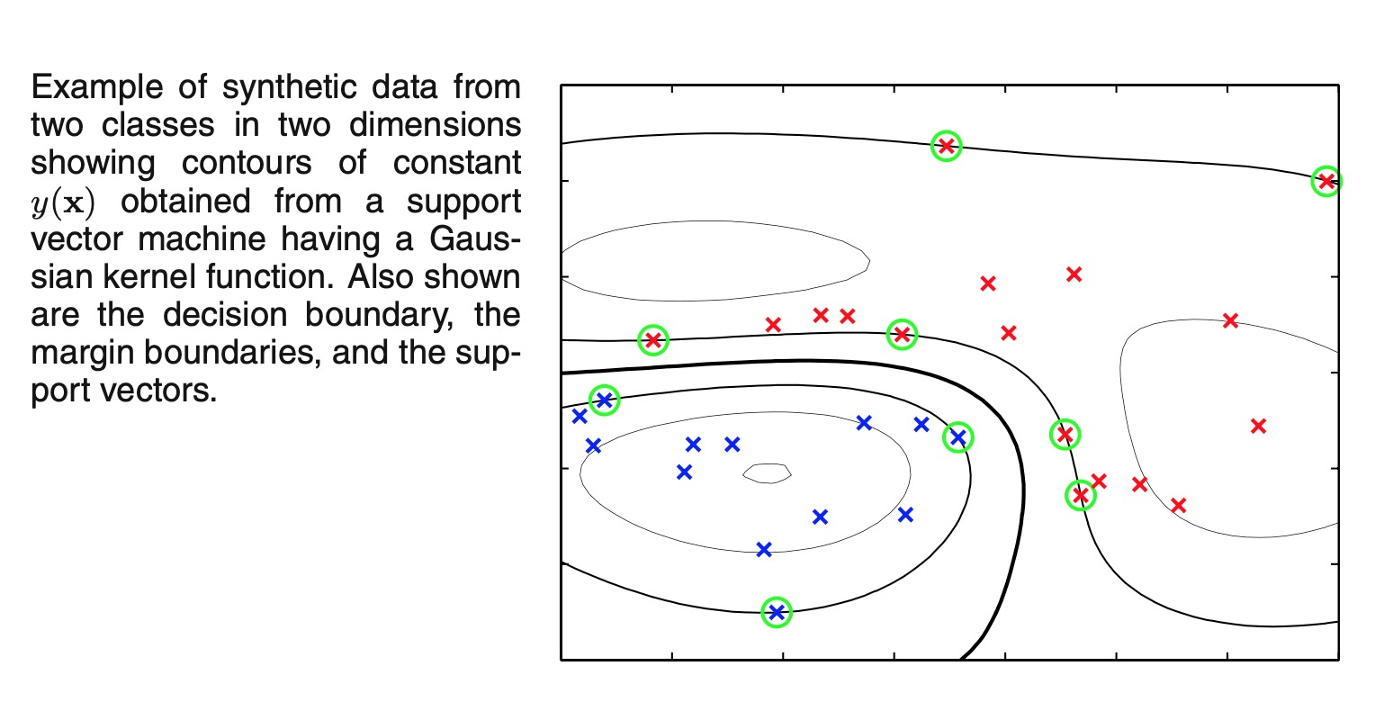
This example also provides a geometrical insight into the origin of sparsity in the SVM. The maximum margin hyperplane is defined by the location of the support vectors. Other data points can be moved around freely (so long as they remain out- side the margin region) without changing the decision boundary, and so the solution will be independent of such data points.

Overlapping class distributions

So far, we have assumed that the training data points are linearly separable in the feature space $\phi(\bold x)$. The resulting support vector machine will give exact separation of the training data in the original input space $\bold x$, although the corresponding decision boundary will be nonlinear. In practice, however, the class-conditional distributions may overlap, in which case exact separation of the training data can lead to poor generalization.

We therefore need a way to modify the support vector machine so as to allow some of the training points to be misclassified. From (7.1.16) we see that in the case of separable classes, we implicitly used an error function that gave infinite error if a data point was misclassified and zero error if it was classified correctly, and then optimized the model parameters to maximize the margin. We now modify this approach so that data points are allowed to be on the ‘wrong side’ of the margin boundary, but with a penalty that increases with the distance from that boundary. For the subsequent optimization problem, it is convenient to make this penalty a linear function of this distance.

Slack Variables

To do this, we introduce slack variables, $\xi_n \ge 0$ where $n = 1, \cdots , N$ with one slack variable for each training data point (Bennett, 1992; Cortes and Vapnik, 1995). These are defined by $\xi_n = 0$ for data points that are on or inside the correct margin boundary and $\xi_n = |t_n − y(\bold x_n)|$ for other points. Thus a data point that is on the decision boundary $y(\bold x_n) = 0$ will have $\xi_n = 1$, and points with $\xi_n \gt 1$ will be misclassified. The exact classification constraints (7.1.5) are then replaced with

$t_ny(\bold x_n) \ge 1 - \xi_n, \hspace{1em} n = 1,\cdots, N \tag{7.1.17}$

in which the slack variables are constrained to satisfy $\xi_n \ge 0$.

Data points for which $\xi_n = 0$ are correctly classified and are either on the margin or on the correct side of the margin. Points for which $0 \lt \xi_n \le 1$ lie inside the margin, but on the correct side of the decision boundary, and those data points for which $\xi_n \gt 1$ lie on the wrong side of the decision boundary and are misclassified, as illustrated in figure below. This is sometimes described as relaxing the hard margin constraint to give a soft margin and allows some of the training set data points to be misclassified. Note that while slack variables allow for overlapping class distributions, this framework is still sensitive to outliers because the penalty for misclassification increases linearly with $\xi$.

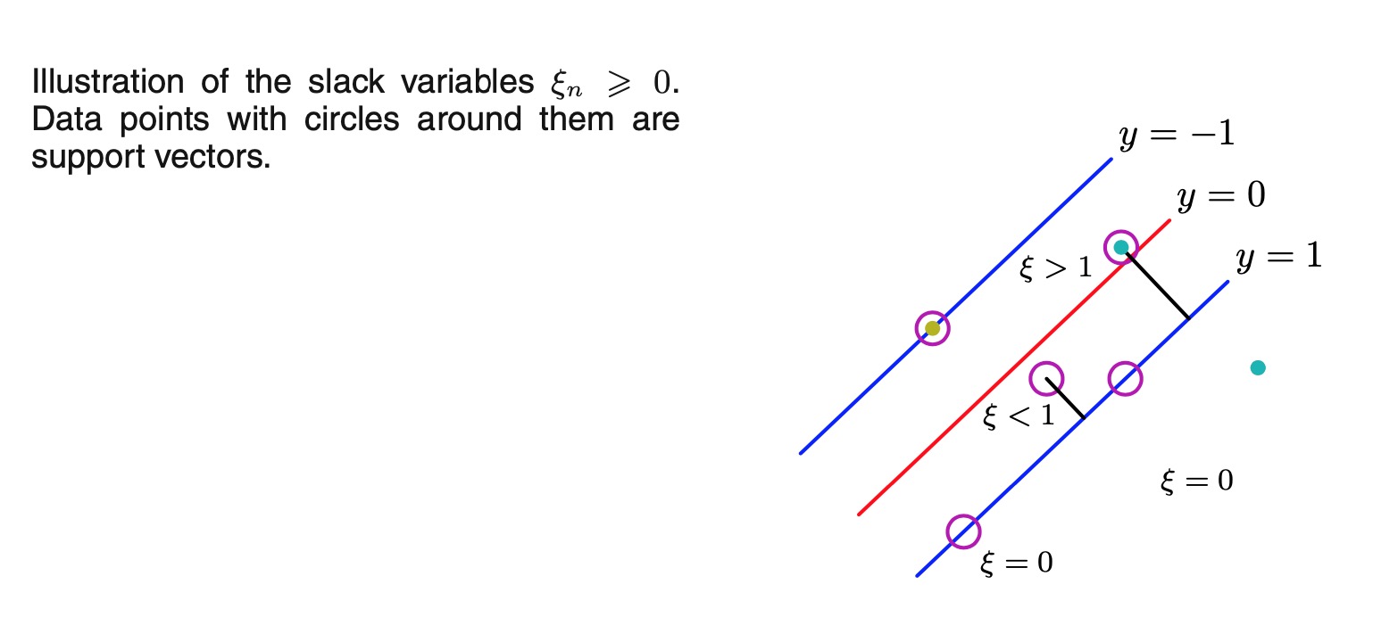
Our goal is now to maximize the margin while softly penalizing points that lie on the wrong side of the margin boundary. We therefore minimize

$C\sum_{n=1}^N\xi_n + \frac{1}{2}||\bold w||^2 \tag{7.1.18}$

where the parameter $C \gt 0$ controls the trade-off between the slack variable penalty and the margin. Because any point that is misclassified has $\xi_n \gt 1$, it follows that $\sum_n\xi_n$ is an upper bound on the number of misclassified points.

The parameter C is therefore analogous to (the inverse of) a regularization coefficient because it controls the trade-off between minimizing training errors and controlling model complexity. In the limit $C \to \infty$, we will recover the earlier support vector machine for separable data.

We now wish to minimize (7.1.18) subject to the constraints (7.1.17) together with $\xi_n \ge 0$. The corresponding Lagrangian is given by

$L(\bold w, b, \bold a) = \frac{1}{2}||\bold w||^2 + C\sum_{n=1}^N\xi_n - \sum_{n=1}^Na_n\{t_ny(\bold x_n) - 1 + \xi_n\} - \sum_{n=1}^N\mu_n\xi_n \tag{7.1.19}$

where $\{a_n \ge 0\}$ and $\{\mu_n \ge 0\}$ are Lagrange multipliers. The corresponding set of KKT conditions are given by

$\begin{aligned}a_n \ge 0 \\ t_ny(\bold x_n) -1 + \xi_n \ge 0 \\ a_n(t_ny(\bold x_n) -1 + \xi_n) = 0 \\ \mu_n \ge 0 \\ \xi_n \ge 0 \\ \mu_x\xi_n \ge 0 \end{aligned} \tag{7.1.20}$

where $n = 1,\cdots, N$.

We now optimize out $\bold w$, b, and $\{xi_n\}$ making use of the definition (7.1,1) of $y(\bold x)$ to give

$\frac{\partial L}{\partial \bold w} = 0 \to \bold w = \sum_{n=1}^Na_nt_n\phi(\bold x_n) \tag{7.1.21}$

$\frac{\partial L}{\partial b} = 0 \to \sum_{n=1}^Na_nt_n =0 \tag{7.1.22}$

$\frac{\partial L}{\partial \xi_n} = 0 \to a_n = C - \mu_n \tag{7.1.23}$

Using these results to eliminate $\bold w$, b, and $\{\xi_n\}$ from the Lagrangian, we obtain the dual Lagrangian in the form

$\widetilde L(\bold a) = \sum_{n=1}^Na_n - \frac{1}{2}\sum_{n=1}^N\sum_{m=1}^Na_na_mt_nt_mk(\bold x_n, \bold x_m) \tag{7.1.24}$

which is identical to the separable case, except that the constraints are somewhat different. To see what these constraints are, we note that $a_n \ge 0$ is required because these are Lagrange multipliers. Furthermore, (7.1.23) together with $\mu_n\ge 0$ implies $a_n \le C$. We therefore have to minimize (7.1.24) with respect to the dual variables $\{a_n\}$ subject to

$0 \le a_n \le C \tag{7.1.25}$

$\sum_{n=1}^Na_nt_n = 0 \tag{7.1.26}$

for $n = 1, . . . , N$ , where (7.1.25) are known as box constraints. This again represents a quadratic programming problem. If we substitute (7.1.21) into (7.1.1), we see that predictions for new data points are again made by using (7.1.12).

Conclusion

We can now interpret the resulting solution. As before, a subset of the data points may have $a_n = 0$, in which case they do not contribute to the predictive model (7.1.12). The remaining data points constitute the support vectors. These have
$a_n \gt 0$ and hence from (7.1.20) must satisfy

$t_ny(\bold x_n) = 1 - \xi_n \tag{7.1.27}$

if $a_n \lt C$, then (7.1.23) implies that $\mu_n \gt 0$, which from (7.1.20) requires $\xi_n = 0$ and hence such points lie on the margin. Points with $a_n = C$ can lie inside the margin and can either be correctly classified if $\xi_n \le 1$ or misclassified if $\xi_n \gt 1$

To determine the parameter b in (7.1.1), we note that those support vectors for which $0<a_n <C$ have $\xi_n =0$ so that $t_ny(\bold x_n)=1$ and hence will satisfy.

$t_n\Bigg(\sum_{m\in S}a_mt_mk(\bold x_n, \bold x_m) + b\Bigg) = 1 \tag{7.1.28}$

Again, a numerically stable solution is obtained by averaging to give

$b = \frac{1}{N_\mathcal{M}} \sum_{n\in \mathcal{M}}\Bigg(t_n - \sum_{m\in S}a_mt_mk(\bold x_n, \bold x_m) \Bigg) \tag{7.1.29}$

where $\mathcal{M}$ denotes the set of indices of data points having $0 < a_n < C$.

Although predictions for new inputs are made using only the support vectors, the training phase (i.e., the determination of the parameters $\bold a$ and b) makes use of the whole data set, and so it is important to have efficient algorithms for solving the quadratic programming problem.

We first note that the objective function $\tilde L(a)$ is quadratic and so any local optimum will also be a global optimum provided the constraints define a convex region (which they do as a consequence of being linear).Direct solution of the quadratic programming problem us- ing traditional techniques is often infeasible due to the demanding computation and memory requirements, and so more practical approaches need to be found. The tech- nique of chunking (Vapnik, 1982) exploits the fact that the value of the Lagrangian is unchanged if we remove the rows and columns of the kernel matrix corresponding to Lagrange multipliers that have value zero. This allows the full quadratic pro- gramming problem to be broken down into a series of smaller ones, whose goal is eventually to identify all of the nonzero Lagrange multipliers and discard the others. Chunking can be implemented using protected conjugate gradients (Burges, 1998). Although chunking reduces the size of the matrix in the quadratic function from the number of data points squared to approximately the number of nonzero Lagrange multipliers squared, even this may be too big to fit in memory for large-scale appli- cations. Decomposition methods (Osuna et al., 1996) also solve a series of smaller quadratic programming problems but are designed so that each of these is of a fixed size, and so the technique can be applied to arbitrarily large data sets. However, it still involves numerical solution of quadratic programming subproblems and these can be problematic and expensive. One of the most popular approaches to training support vector machines is called sequential minimal optimization, or SMO (Platt, 1999). It takes the concept of chunking to the extreme limit and considers just two Lagrange multipliers at a time. In this case, the subproblem can be solved analyti- cally, thereby avoiding numerical quadratic programming altogether. Heuristics are given for choosing the pair of Lagrange multipliers to be considered at each step. In practice, SMO is found to have a scaling with the number of data points that is somewhere between linear and quadratic depending on the particular application.

inner product kernel

We have seen that kernel functions correspond to inner products in feature spaces that can have high, or even infinite, dimensionality. By working directly in terms of the kernel function, without introducing the feature space explicitly, it might there- fore seem that support vector machines somehow manage to avoid the curse of dimensionality.

This is not the case, however, because there are constraints amongst the feature values that restrict the effective dimensionality of feature space. To see this consider a simple second-order polynomial kernel that we can expand in terms of its components
${}k(\bold x, \bold z) \\ = (1+\bold x^T\bold z)^2 \\ = (1 + x_1z_1 + x_2z_2)^2 \\ = 1 + 2x_1z_1 + 2x_2z_2 + x_1^2z_1^2 + 2x_1z_1x_2z_2 + x_2^2z_2^2 \\ = (1, \sqrt{2}x_1, \sqrt{2}x_2, x_1^2, \sqrt{2}x_1x_2, x_2^2)(1,\sqrt{2}z_1, \sqrt{2}z_2, z_1^2, \sqrt{2}z_1z_2, z_2^2)^T \\ = \phi(\bold x)^T\phi(\bold z)$

This kernel function therefore represents an inner product in a feature space having six dimensions, in which the mapping from input space to feature space is described by the vector function $\phi(\bold x)$. However, the coefficients weighting these different features are constrained to have specific forms. Thus any set of points in the original two-dimensional space $\bold x$ would be constrained to lie exactly on a two-dimensional nonlinear manifold embedded in the six-dimensional feature space.

We have already highlighted the fact that the support vector machine does not provide probabilistic outputs but instead makes classification decisions for new input vectors. Veropoulos et al. (1999) discuss modifications to the SVM to allow the trade-off between false positive and false negative errors to be controlled. However, if we wish to use the SVM as a module in a larger probabilistic system, then probabilistic predictions of the class label t for new inputs x are required.

To address this issue, Platt (2000) has proposed fitting a logistic sigmoid to the outputs of a previously trained support vector machine. Specifically, the required conditional probability is assumed to be of the form

$p(t=1|\bold x) = \sigma(Ay(\bold x) + B)$

where $y(\bold x)$ is defined by (7.1.1). Values for the parameters A and B are found by minimizing the cross-entropy error function defined by a training set consisting of pairs of values $y(\bold x_n)$ and $t_n$. The data used to fit the sigmoid needs to be independent of that used to train the original SVM in order to avoid severe over-fitting. This two-stage approach is equivalent to assuming that the output $y(\bold x)$ of the support vector machine represents the log-odds of $\bold x$ belonging to class $t = 1$. Because the SVM training procedure is not specifically intended to encourage this, the SVM can give a poor approximation to the posterior probabilities (Tipping, 2001).

Relation to logistic regression

As with the separable case, we can re-cast the SVM for nonseparable distri- butions in terms of the minimization of a regularized error function. This will also allow us to highlight similarities, and differences, compared to the logistic regression model.

We have seen that for data points that are on the correct side of the margin boundary, and which therefore satisfy $y_nt_n \ge 1$, we have $\xi_n = 0$, and for the remaining points we have $\xi_n = 1 − y_nt_n$. Thus the objective function (7.1.18) can be written (up to an overall multiplicative constant) in the form

$\sum_{n=1}^NE_{SV} (y_nt_n) + \lambda||\bold w||^2 \tag{7.1.30}$

where $\lambda = (2C)^{-1}$ and $E_{SV}(\cdot)$ is the hinge error function defined by

$E_{SV}(y_nt_n) = [1-y_nt_n]_+ \tag{7.1.31}$

where $[ \cdot ]_+$ denotes the positive part. The hinge error function, so-called because of its shape, is plotted as follow.
It can be viewed as an approximation to the misclassification error, i.e., the error function that ideally we would like to minimize, which is also shown in Figure

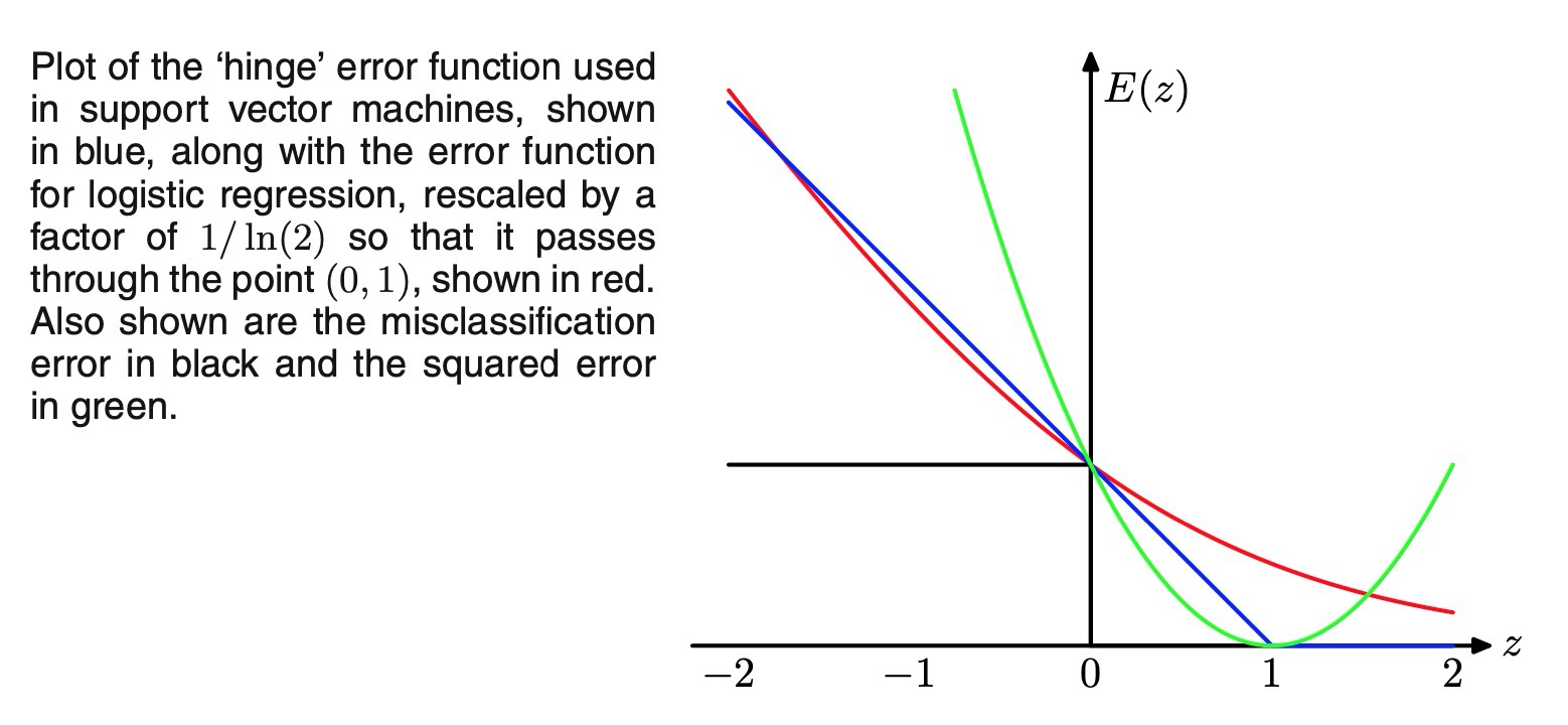
When we considered the logistic regression model in Section 4.3.2, we found it convenient to work with target variable $t \in \{0, 1\}$. For comparison with the support vector machine, we first reformulate maximum likelihood logistic regression using the target variable $t \in \{−1, 1\}$.

To do this, we note that $p(t = 1|y) = σ(y)$ where $y(\bold x)$ is given by (7.1.1), and $\sigma(y)$ is the logistic sigmoid function. It follows that $p(t = −1|y) = 1 − \sigma(y) = \sigma(−y)$, where we have used the properties of the logistic sigmoid function, and so we can write

$p(t|y) = \sigma(yt) \tag{7.1.32}$

From this we can construct an error function by taking the negative logarithm of the likelihood function that, with a quadratic regularizer, takes the form

$\sum_{n=1}^NE_{LR}(y_nt_n) + \lambda||\bold w||^2 \tag{7.1.33}$

where

$E_{LR}(yt) = ln (1 + exp(−yt)) \tag{7.1.34}$

For comparison with other error functions, we can divide by $ln(2)$ so that the error function passes through the point (0, 1). This rescaled error function is also plotted in Figure above and we see that it has a similar form to the support vector error function. The key difference is that the flat region in $E_{SV}(yt)$ leads to sparse solutions.

Error Function Comparison

Both the logistic error and the hinge loss can be viewed as continuous approx- imations to the misclassification error. Another continuous error function that has sometimes been used to solve classification problems is the squared error, which is again plotted in Figure above. It has the property, however, of placing increasing emphasis on data points that are correctly classified but that are a long way from the decision boundary on the correct side. Such points will be strongly weighted at the expense of misclassified points, and so if the objective is to minimize the mis- classification rate, then a monotonically decreasing error function would be a better choice.

Multiclass SVMs

The support vector machine is fundamentally a two-class classifier. In practice, however, we often have to tackle problems involving K > 2 classes. Various meth- ods have therefore been proposed for combining multiple two-class SVMs in order to build a multiclass classifier.

SVMs for regression

We now extend support vector machines to regression problems while at the same time preserving the property of sparseness.
In simple linear regression, we minimize a regularized error function given by

$\displaystyle \frac{1}{2}\sum_{n=1}^N\{y_n - t_n\}^2 + \frac{\lambda}{2}||\bold w||^2$

To obtain sparse solutions, the quadratic error function is replaced by an $\varepsilon$-insensitive error function (Vapnik, 1995), which gives zero error if the absolute difference between the prediction $y(\bold x)$ and the target t is less than $\varepsilon$ where $\varepsilon \gt 0$. A simple example of an $\varepsilon$-insensitive error function, having a linear cost associated with errors outside the insensitive region, is given by

$E_\varepsilon(y(\bold x) - t) = \begin{cases} 0, & \text{if } |y(\bold x) -t| \lt \varepsilon \\ |y(\bold x) - t| - \varepsilon, & otherwise \end{cases} \tag{7.1.35}$

and is illustrated in Figure follow

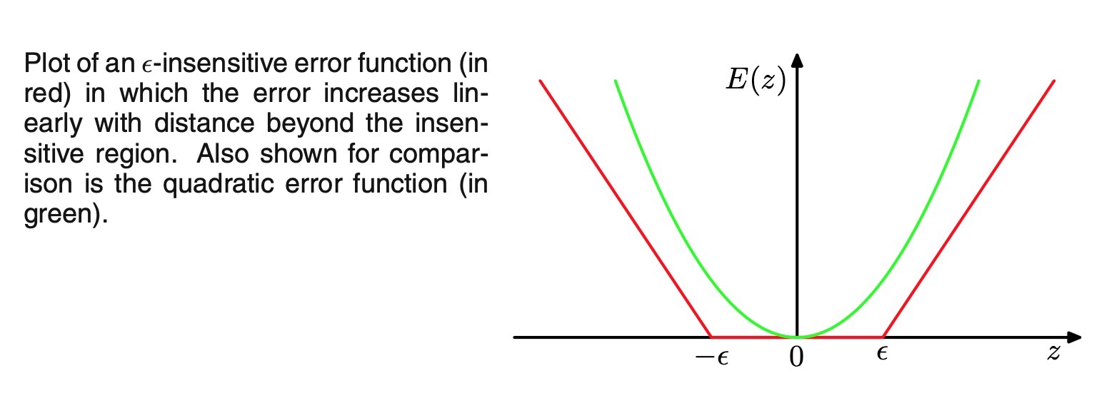
We therefore minimize a regularized error function given by

$C\sum_{n=1}^NE_\varepsilon(y(\bold x_n) - t_n) + \frac{1}{2}||\bold w||^2\tag{7.1.36}$

where $y(\bold x)$ is given by (7.1.1). By convention the (inverse) regularization parameter, denoted C, appears in front of the error term.

As before, we can re-express the optimization problem by introducing slack variables. For each data point $\bold x_n$, we now need two slack variables $\xi_n \ge 0$ and $\hat \xi_n \ge 0$, where $\xi_n \ge 0$ corresponds to a point for which $t_n \gt y(\bold x_n)+\varepsilon$,and $\hat\xi_n \gt 0$ corresponds to a point for which $t_n \lt y(\bold x_n) − \varepsilon$, as illustrated in Figure follow.

The condition for a target point to lie inside the $\varepsilon$-tube is that $y_n − \varepsilon \le t_n \le y_n + \varepsilon$, where $y_n = y(\bold x_n)$. Introducing the slack variables allows points to lie outside the tube provided the slack variables are nonzero, and the corresponding conditions are

$\begin{cases} t_n \le y(\bold x_n) + \varepsilon + \xi_n \\ t_n \ge y(\bold x_n) - \varepsilon - \hat\xi_n\end{cases} \tag{7.1.37}$

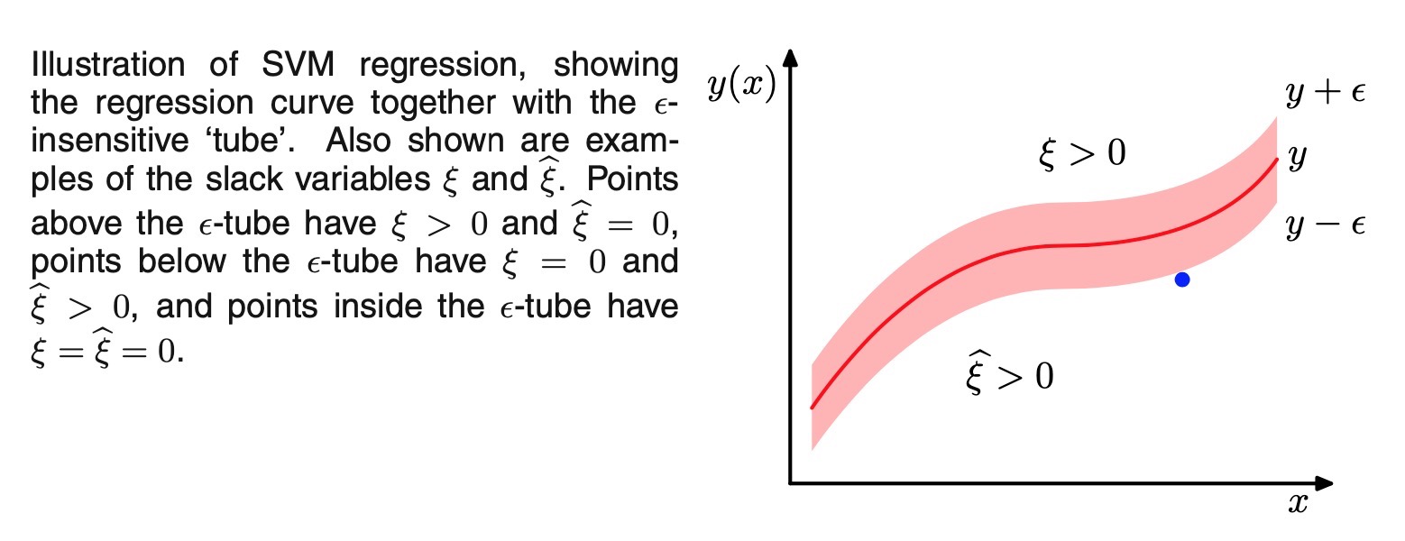
The error function for support vector regression can then be written as

$C\sum_{n=1}^N(\xi_n + \hat\xi_n) + \frac{1}{2}||\bold w||^2 \tag{7.1.38}$

which must be minimized subject to the constraints $\xi_n \ge 0$ and $\hat\xi_n \ge 0$ and the (7.1.37).
This can be achieved by introducing Lagrange multipliers $a_n \ge 0, \hat a_n \ge 0, \mu_n \ge 0, \hat\mu_n \ge 0$ and optimizing the Lagrangian

$L = C\sum_{n=1}^N(\xi_n + \hat\xi_n) + \frac{1}{2}||\bold w||^2 - \sum_{n=1}^N(\mu_n\xi_n + \hat\mu_n\hat\xi_n) \\ - \sum_{n=1}^Na_n(\varepsilon + \xi_n + y_n - t_n) \\ - \sum_{n=1}^N\hat a_n(\varepsilon + \hat\xi_n - y_n + t_n) \tag{7.1.39}$

We now substitute for y(x) using (7.1.1) and then set the derivatives of the Lagrangian with respect to $\bold w$, b, $\xi$, and $\hat\xi_n$ to zero, giving

$\frac{\partial L}{\partial \bold w} = 0 \to \bold w = \sum_{n=1}^N(a_n - \hat a_n)\phi(\bold x_n) \tag{7.1.40}$

$\frac{\partial L}{\partial b} = 0 \to \sum_{n=1}^N(a_n - \hat a_n) = 0 \tag{7.1.41}$

$\frac{\partial L}{\partial \xi_n} = 0 \to a_n + \mu_n = C \tag{7.1.42}$

$\frac{\partial L}{\partial \hat\xi_n} = 0 \to \hat a_n + \hat\mu_n = C \tag{7.1.43}$

Using these results to eliminate the corresponding variables from the Lagrangian, we see that the dual problem involves maximizing

$\tilde{L}(\bold a, \hat\bold a) = -\frac{1}{2}\sum_{n=1}^N\sum_{n=1}^N(a_n - \hat a_n)(a_m - \hat a_m)k(\bold x_n, \bold x_m) \\ - \varepsilon\sum_{n=1}^N(a_n + \hat a_n) + \sum_{n=1}^N(a_n - \hat a_n)t_n \tag{7.1.44}$

with respect to $\{a_n\}$ and $\{\hat a_n\}$, where we have introduced the kernel $k(\bold x,\bold x') = \phi(\bold x)^T\phi(\bold x')$.

Again, this is a constrained maximization, and to find the constraints we note that $a_n \ge 0$ and $\hat a_n \ge 0$ are both required because these are Lagrange multipliers. Also $\mu_n \ge 0$ and $\hat\mu_n \ge 0$ together with (7.1.42) and (7.1.43), require $a_n \le C$ and $\hat a_n \le C$, and so again we have the box constraints

$\begin{cases} 0 \le a_n \le C \\ 0 \le \hat a_n \le C \end{cases} \tag{7.1.45}$

together with the condition (7.1.41).

Substituting (7.1.40) into (7.1.1), we see that predictions for new inputs can be made

$y(\bold x) = \sum_{n=1}^N(a_n - \hat a_n)k(\bold x, \bold x_n) + b \tag{7.1.46}$

which is again expressed in terms of the kernel function.
The corresponding Karush-Kuhn-Tucker (KKT) conditions, which state that at
the solution the product of the dual variables and the constraints must vanish, are given by

$\begin{aligned}a_n(\varepsilon + \xi_n + y_n - t_n) = 0 \\ \hat a_n(\varepsilon + \hat\xi_n - y_n + t_n) = 0 \\ (C - a_n)\xi_n = 0 \\ (C-\hat a_n)\hat\xi_n = 0\end{aligned} \tag{7.1.47}$

From these we can obtain several useful results.

First of all, we note that a coefficient an can only be nonzero if $\varepsilon+\xi_n +y_n −t_n =0$,which implies that the data point either lies on the upper boundary of the $\varepsilon$-tube ($\xi_n = 0$) or lies above the upper boundary ($\xi_n > 0$).
Similarly, a nonzero value for an implies $\varepsilon + \hat\xi_n − y_n + t_n = 0$, and such points must lie either on or below the lower boundary of the $\varepsilon$-tube.
Furthermore, the two constraints $\varepsilon+\xi_n +y_n −t_n =0$ and $\varepsilon + \hat\xi_n − y_n + t_n = 0$ are incompatible, as is easily seen by adding them together and noting that $\xi_n$ and $\hat\xi_n$ are nonnegative while $\varepsilon$ is strictly positive, and so for every data point $\bold x_n$, either $a_n$ or $\hat a_n$ (or both) must be zero.

The support vectors are those data points that contribute to predictions given by (7.1.46), in other words those for which either an $a_n \ne 0$ or $\hat a_n \ne 0$. These are points that lie on the boundary of the $\varepsilon$-tube or outside the tube. All points within the tube have $a_n = \hat a_n = 0$. We again have a sparse solution, and the only terms that have to be evaluated in the predictive model (7.1.46) are those that involve the support vectors.

The parameter $b$ can be found by considering a data point for which $0 < a_n < C$, which from (7.1.47- line 3) must have $\xi_n = 0$, and from (7.1.47-line 1) must therefore satisfy $\varepsilon + y_n − t_n = 0$. Using (7.1.1) and solving for $b$, we obtain

$b = t_n - \varepsilon - \bold w^T\phi(\bold x_n) = t_n - \varepsilon - \sum_{m=1}^N(a_m - \hat a_m)k(\bold x_n, \bold x_m) \tag{7.1.48}$

where we have used (7.1.40). We can obtain an analogous result by considering a point for which $0 < \hat a_n < C$. In practice, it is better to average over all such estimates of b.

Computational learning theory

[Skip]

Relevance Vector Machines

[TODO]

Graphical Models

We shall find it highly advantageous to augment the analysis using diagrammatic representations of probability distributions, called probabilistic graphical models. These offer several useful properties:

1. They provide a simple way to visualize the structure of a probabilistic model and can be used to design and motivate new models.

2. Insights into the properties of the model, including conditional independence properties, can be obtained by inspection of the graph.

3. Complex computations, required to perform inference and learning in sophis- ticated models, can be expressed in terms of graphical manipulations, in which underlying mathematical expressions are carried along implicitly.

A graph comprises nodes (also called vertices) connected by links (also known as edges or arcs). In a probabilistic graphical model, each node represents a random variable (or group of random variables), and the links express probabilistic relationships between these variables. The graph then captures the way in which the joint distribution over all of the random variables can be decomposed into a product of factors each depending only on a subset of the variables.

We shall begin by discussing Bayesian networks, also known as directed graphical models, in which the links of the graphs have a particular directionality indicated by arrows. The other major class of graphical models are Markov random fields, also known as undirected graphical models, in which the links do not carry arrows and have no directional significance. Directed graphs are useful for expressing causal relationships between random variables, whereas undirected graphs are better suited to expressing soft con- straints between random variables. For the purposes of solving inference problems, it is often convenient to convert both directed and undirected graphs into a different representation called a factor graph.

Bayesian Networks

[TODO]

Conditional Independence

An important concept for probability distributions over multiple variables is that of conditional independence.

Markov Random Fields

We have seen that directed graphical models specify a factorization of the joint dis- tribution over a set of variables into a product of local conditional distributions. They also define a set of conditional independence properties that must be satisfied by any distribution that factorizes according to the graph. We turn now to the second ma- jor class of graphical models that are described by undirected graphs and that again specify both a factorization and a set of conditional independence relations.

A Markov random field, also known as a Markov network or an undirected graphical model (Kindermann and Snell, 1980), has a set of nodes each of which corresponds to a variable or group of variables, as well as a set of links each of which connects a pair of nodes. The links are undirected, that is they do not carry arrows. In the case of undirected graphs, it is convenient to begin with a discussion of conditional independence properties.

Inference in Graphical Models

We turn now to the problem of inference in graphical models, in which some of the nodes in a graph are clamped to observed values, and we wish to compute the posterior distributions of one or more subsets of other nodes.

we can exploit the graphical structure both to find efficient algorithms for inference, and to make the structure of those algorithms transparent. Specifically, we shall see that many algorithms can be expressed in terms of the propagation of local messages around the graph. In this section, we shall focus primarily on techniques for exact inference

Mixture Models and EM

If we define a joint distribution over observed and latent variables, the corresponding distribution of the observed variables alone is obtained by marginalization. This allows relatively complex marginal distributions over observed variables to be expressed in terms of more tractable joint distributions over the expanded space of observed and latent variables. The introduction of latent variables thereby allows complicated distributions to be formed from simpler components.

In this section, we shall see that mixture distributions, such as the Gaussian mixture discussed in Section 2.3.9, can be interpreted in terms of discrete latent variables. Continuous latent variables will form the subject of Section 12.

As well as providing a framework for building more complex probability dis- tributions, mixture models can also be used to cluster data. We therefore begin our discussion of mixture distributions by considering the problem of finding clusters in a set of data points, which we approach first using a nonprobabilistic technique called the K-means algorithm (Lloyd, 1982). Then we introduce the latent variable view of mixture distributions in which the discrete latent variables can be interpreted as defining assignments of data points to specific components of the mixture. A gen- eral technique for finding maximum likelihood estimators in latent variable models is the expectation-maximization (EM) algorithm. We first of all use the Gaussian mixture distribution to motivate the EM algorithm in a fairly informal way, and then we give a more careful treatment based on the latent variable viewpoint. We shall see that the K-means algorithm corresponds to a particular nonprobabilistic limit of EM applied to mixtures of Gaussians. Finally, we discuss EM in some generality.

Gaussian mixture models are widely used in data mining, pattern recognition, machine learning, and statistical analysis. In many applications, their parameters are determined by maximum likelihood, typically using the EM algorithm.

K-means Clustering

[TODO]

Mixtures of Gaussians

[TODO]

An Alternative View of EM

[TODO]

The EM Algorithm in General

[TODO]

Approximate Inference

[SKIP]

Sampling Methods

[VIP_TODO]
For most probabilistic models of practical interest, exact inference is intractable, and so we have to resort to some form of approximation. Here we consider approximate inference methods based on numerical sampling, also known as Monte Carlo techniques.

Although for some applications the posterior distribution over unobserved variables will be of direct interest in itself, for most situations the posterior distribution is required primarily for the purpose of evaluating expectations, for example in order to make predictions. The fundamental problem that we therefore wish to address in this chapter involves finding the expectation of some function f (z) with respect to a probability distribution p(z). Here, the components of z might comprise discrete or continuous variables or some combination of the two.

Thus in the case of continuous variables, we wish to evaluate the expectation

$E[f] = \int f(\bold z)p(\bold z)d\bold z\tag{11.1.1}$

where the integral is replaced by summation in the case of discrete variables. This is illustrated schematically for a single continuous variable in Figure 11.1. We shall suppose that such expectations are too complex to be evaluated exactly using analyt- ical techniques.

Basic Sampling Algorithms

Markov Chain Monte Carlo

Gibbs Sampling

Slice Sampling

The Hybrid Monte Carlo Algorithm

Estimating the Partition Function

Continuous Latent Variables

[TODO_VIP]

Principal Component Analysis

Probabilistic PCA

Kernel PCA

Nonlinear Latent Variable Models

Sequential Data

[TODO_VIP]

Markov Models

Hidden Markov Models

Linear Dynamical Systems

Combining Models

[SKIP]

@Reference

• Pattern Recognition And Maching Learning by Christopher M. Bishop
• how-to-derive-the-mean-and-variance-of-a-gaussian-random-variable