Computer Vision Algorithms And Applications(计算机视觉算法与应用)

Image Proccessing

Point Operators

@(Point Operators)[pixel||color|compositing]

@(Pixel)

Two commonly used point processes are multiplication and addition with a constant

$g(x) = af (x) + b \tag{1.0.1}$

The parameters $a > 0$ and $b$ are often called the gain and bias parameters; sometimes these parameters are said to control contrast and brightness.
The bias and gain parameters can also be spatially varying $g(x) = a(x)f(x) + b(x)$

Multiplicative gain (both global and spatially varying) is a linear operation, since it obeys the superposition principle $h(f_0 + f_1) = h(f_0) + h(f_1)$

Another commonly used dyadic (two-input) operator is the linear blend operator

$g(x) = (1-\alpha)f_0(x) + \alpha f_1(x) \tag{1.0.2}$

@(Compositing and matting)

Compositing equation $C = (1-\alpha)B + \alpha F$.

This operator attenuates the influence of the background image B by a factor (1 − α) and then adds in the color (and opacity) values corresponding to the foreground layer F

Linear Filtering

The most commonly used type of neighborhood operator is a linear filter, in which an output pixel’s value is determined as a weighted sum of input pixel values

$\displaystyle g(i,j) = \sum_{k,l}f(i+k, j+l)h(k,l) \tag{1.0.1}$

The entries in the weight kernel or mask h(k, l) are often called the filter coefficients. The above correlation operator can be more compactly notated as $g = f\otimes h$

A common variant on this formula is

$\displaystyle g(i,j) = \sum_{k,l}f(i-k,j-l)h(k,l) = \sum_{k,l}f(k,l)h(i-k, j-l) \tag{1.0.2}$

where the sign of the offsets in f has been reversed. This is called the convolution operator, $g = f*h$

@(Separable filtering)

The process of performing a convolution requires $K^2$ (multiply-add) operations per pixel, where $K$ is the size (width or height) of the convolution kernel. In many cases, this operation can be significantly sped up by first performing a one-dimensional horizontal convolution followed by a one-dimensional vertical convolution (which requires a total of 2K operations per pixel). A convolution kernel for which this is possible is said to be separable.
It is easy to show that the two-dimensional kernel K corresponding to successive con- volution with a horizontal kernel h and a vertical kernel v is the outer product of the two kernels
K = vh^T \tag{1.0.3}

How can we tell if a given kernel $K$ is indeed separable? This can often be done by inspection or by looking at the analytic form of the kernel. A more direct method is to treat the 2D kernel as a 2D matrix K and to take its singular value decomposition (SVD)

$\displaystyle K = \sum_i\sigma_iu_iv_i^T \tag{1.0.4}$

If only the first singular value $\sigma_0$ is non-zero, the kernel is separable and $\sqrt{\sigma_0}u_0$ and $\sqrt{\sigma_0}v_0^T$ provide the vertical and horizontal kernels (Perona 1995). For example, the Laplacian of Gaussian kernelcan be implemented as the sum of two separable filters.

@(Operator)[sobel|corner|gaussian]

1. Sobel Operator

$\frac{1}{8} \begin{bmatrix} -1 & 0 & -1 \\ -2 & 0 & -2 \\ -1 & 0 & -1\end{bmatrix} \hspace {2em} \frac{1}{8} \begin{bmatrix}1 & 2 & 1\\ 0 & 0 & 0 \\ -1 & -2 & -1 \end{bmatrix}$

Sobel算子考虑了水平、垂直和2个对角共计4个方向对的梯度加权求和，是一个3×3各向异性的梯度算子。
Sobel算子具有严格的数学基础，主要关键点在于

1. Cartesian grid
2. Forward-difference
3. the distance inverse ratio weighted sum of gradient along the 4 direction
4. City-block distance (Neihtor Checkboard distance Nor Euclidean distance)
   the neighborhood domain gradient vector g level define as $g = \frac{\text{density difference}}{\text{distance to neighbor}}$
   So for the neighorbood N8 domain $\def\arraystretch{1.0} \begin{array}{c:c:c} z_1& z_2 & z_3 \\ \hline z_4 & z_5 & z_6 \\ \hdashline z_7 & z_8 & z_9 \end{array}$
   Along the 4 direction $(z_1, z_9) ，(z_2, z_8)， (z_3, z_7)， (z_6, z_4)$ gets the sum gradient to esimate the $z_5$
   $G = \frac{z_3-z_7}{4} * [1, 1]+ \frac{z_1-z_9}{4}* [-1, 1] + \frac{z_2-z_8}{2}* [0, 1]+ \frac{z_6-z_4}{2}* [1, 0]$
   $G = [\frac{z_3- z_7- z_1+ z_9}{4} + \frac{z_6-z_4}{2}, \frac{z_3- z_7+ z_1- z_9}{4} + \frac{z_2-z_8}{2}]$
   let $G' = 4G \to \begin{cases}G'_x = (z_3 + 2*z_6 + z_9) - (z_1 + 2*z_4 + z_7)\\ G'_y = (z_1 + 2*z_2 + z_3) - (z_7 + 2*z_8 + z_9)\end{cases}$

2. corner Operator

$\frac{1}{4}\begin{bmatrix}1 & -2 & 1\\ -2 & 4 & -2\\ 1 & -2 & 1\end{bmatrix}$

@(linear filtering)[lowpass|highpass]

Smoothing kernels can also be used to sharpen images using a process called unsharp masking. Since blurring the image reduces high frequencies, adding some of the difference between the original and the blurred image makes it sharper

$\displaystyle \begin{cases}g_{sharp} = f + \gamma(f - h_{blur} * f) \\ g_{unsharp} = f(1 - \gamma h_{blur} * f)\end{cases}\tag{1.0.5}$

@(Band-pass and steerable filters)[Gaussian filter | Laplacian operator]

The Sobel and corner operators are simple examples of band-pass and oriented filters.More sophisticated kernels can be created by first smoothing the image with a (unit area) Gaussian filter and then taking the first or second derivatives.

$G(x,y; \sigma) = \frac{1}{2\pi\sigma^2} e^{-\frac{x^2 + y^2}{2\sigma^2}}\tag{1.0.6}$

Such filters are known collectively as band-pass filters, since they filter out both low and high frequencies.

The (undirected) second derivative of a two-dimensional image $\nabla^2 f = \frac{\partial^2 f}{\partial x^2} + \frac{\partial^2 f}{\partial y^2}$ is known as the Laplacian operator.
Blurring an image with a Gaussian and then taking its Laplacian is equivalent to convolving directly with the Laplacian of Gaussian (LoG) filter as follow

$\displaystyle \nabla^2G(x,y;\sigma) = \bigg(\frac{x^2 + y^2}{\sigma^4} - \frac{2}{\sigma^2}\bigg)G(x,y;\sigma) \tag{1.0.7}$

Pyramids and wavelets

@(Pyramids and wavelets)[Gaussion pyramid | Laplace pyramid Blending]

In order to interpolate (or upsample) an image to a higher resolution, we need to select some interpolation kernel with which to convolve the image

$\displaystyle g(i,j) = \sum_{k,l}f(k,l)h(i-rk, j - rl) \tag{1.0.8}$

where r is the upsampling rate

While interpolation can be used to increase the resolution of an image, decimation (downsampling) is required to reduce the resolution. To perform decimation, we first (conceptually) convolve the image with a low-pass filter to avoid aliasing) and then keep every $r$th sample.

$\displaystyle g(i,j) = \sum_{k,l}f(k,l)h(ri-k,rj-l) = \frac{1}{r}\sum_{k,l}f(k,l)h(i-k/r, j-l/r)\tag{1.0.9}$

Now that we have described interpolation and decimation algorithms, we can build a complete image pyramid. As we mentioned before, pyramids can be used to accelerate coarse-to-fine search algorithms, to look for objects or patterns at different scales, and to perform multi-resolution blending operations.

Gaussian Pyramid Imagine the pyramid as a set of layers in which the higher the layer, the smaller the size. Every layer is numbered from bottom to top, so layer $(i+1)$ (denoted as $G_{i+1}$ is smaller than layer $i (G_{i}$).

Constructing the Gaussian pyramid (Used to downsample images)

1. Convolve $G_{i}$ with a Gaussian kernel: $\frac{1}{256}\begin{bmatrix}1 & 4 & 6 & 4 & 1\\ 4 & 16 & 24 & 16 & 4 \\ 6 & 24 & 36 & 24 & 6 \\4 & 16 & 24 & 16 & 4 \\ 1 & 4 & 6 & 4 & 1 \end{bmatrix}$
2. Remove every even-numbered row and column.
3. Redo step 1 and step 2 to procedure layer $G_{i + 1}$

Constructing the Laplacian pyramid (Used to reconstruct an upsampled image from an image lower in the pyramid (with less resolution))

$L_i = G_i - Up(G_{i + 1})\otimes K_{5x5}$

$G_i$ is the layer $i$ Gaussian pyramid image, $G_{i + 1}$ is layer $i + 1$. $Up$ is the upsample

Application: Image Blending

@(Application)[Image Blending]

One of the most engaging and fun applications of the Laplacian pyramid presented is the creation of blended composite images.

Geometric transformations

@(Geometric transformations)

1. parametric transformations, such as translation, rigid, similarity, affine, projective.
2. Mesh-based warping

Application: Feature-based morphing

While warps can be used to change the appearance of or to animate a single image, even more powerful effects can be obtained by warping and blending two or more images using a process now commonly known as morphing.

Global optimization

MRF-Markov Random Field

Feature detection and matching

Points and patches

There are two main approaches to finding feature points and their correspondences.

1. Finding features in one image that can be accurately tracked using a local search technique, such as correlation or least squares
2. Independently detect features in all the images under consideration and then match features based on their local appearance

The keypoint detection and matching pipeline can be split into four separate stages.

1. feature detection (extraction) stage.
   Each image is searched for locations that are likely to match well in other images.
2. feature description stage
   Each region around detected keypoint locations is converted into a more compact and stable (invariant) descriptor that can be matched against other descriptors.
3. feature matching stage
   Efficiently searches for likely matching candidates in other images.
4. feature tracking stage
   It’s an alternative to the third stage that only searches a small neighborhood around each detected feature and is therefore more suitable for video processing.

Feature detectors

@[Feature detectors]

Patches with large contrast changes (gradients) are easier to localize, although straight line segments at a single orientation suffer from the aperture problem. Patches with gradients in at least two (significantly) different orientations are the easiest to localize

These intuitions can be formalized by looking at the simplest possible matching criterion for comparing two image patches, i.e., their (weighted) summed square difference

$\displaystyle E_{WSSD}(\mathbf u) = \sum_{i}\omega(x_i)[I_1(x_i + \mathbf u) - I_0(x_i)]^2 \tag{2.0.1}$

where $I_0$ and $I_1$ are the two images being compared, $\mathbf u = (u, v)$ is the displacement vector, $\omega(x)$ is a spatially varying weighting (or window) function, and the summation $i$ is over all the pixels in the patch. Note that the same formulation can also used to estimate motion between complete images.

When performing feature detection, we do not know which other image locations the feature will end up being matched against. Therefore, we can only compute how stable this metric is with respect to small variations in position $\Delta u$ by comparing an image patch against itself, which is known as an auto-correlation function or surface

$E_{AC}(\Delta u) = \sum_i\omega(x_i)[I_0(x_i + \Delta u) - I_0(x_i)]^2 \tag{2.0.2}$

Using a Taylor Series expansion of the image function $I_0(x_i +\Delta u) \approx I_0(x_i) + \nabla I_0(x_i)\cdot \Delta u$ (Lucas and Kanade 1981; Shi and Tomasi 1994), we can approximate the auto-correlation surface as

$E_{AC}(\Delta u) = \sum_i\omega(x_i)[I_0(x_i + \Delta u) - I_0(x_i)]^2\\ \approx \sum_i\omega(x_i)[I_0(x_i) + \nabla I_0(x_i)\cdot \Delta u - I_0(x_i)]^2\\ = \sum_i\omega(x_i)[\nabla I_0(x_i)\cdot\Delta u]^2 = \Delta u^TA\Delta u \tag{2.0.3}$

where $\nabla I_0(x_i) = (\frac{\partial I_0}{\partial x}, \frac{\partial I_0}{\partial y})(x_i)$ is the image gradient at $x_i$. This gradient can be computed using a variety of techniques (Schmid, Mohr, and Bauckhage 2000).

The classic “Harris” detector (Harris and Stephens 1988) uses a $[-2\space -1\space 0\space 1\space 2]$ filter, but more modern variants (Schmid, Mohr, and Bauckhage 2000; Triggs 2004) convolve the image with horizontal and vertical derivatives of a Gaussian (typically with $\sigma = 1$).

The auto-correlation matrix $A$ can be written as $A = \omega\begin{bmatrix}I_x^2 & I_xI_y \\ I_xI_y & I_y^2\end{bmatrix}$ where we have replaced the weighted summations with discrete convolutions with the weight- ing kernel $\omega$. This matrix can be interpreted as a tensor (multiband) image, where the outer products of the gradients $\nabla I$ are convolved with a weighting function $\omega$ to provide a per-pixel estimate of the local (quadratic) shape of the auto-correlation function.

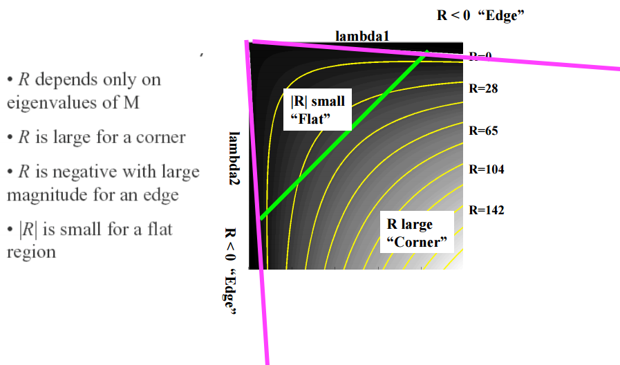
The inverse of the matrix A provides a lower bound on the uncertainty in the location of a matching patch. It is therefore a useful indicator of which patches can be reliably matched. The easiest way to visualize and reason about this uncertainty is to perform an eigenvalue analysis of the auto-correlation matrix $A$, which produces two eigenvalues ($\lambda_0 , \lambda_1$ ) and two eigenvector directions.

Since the larger uncertainty depends on the smaller eigenvalue, it makes sense to find maxima in the smaller eigenvalue to locate good features to track.

@(Fo ̈rstner–Harris)

While Anandan and Lucas and Kanade(1981)were the first to analyze the uncertainty structure of the auto-correlation matrix, they did so in the context of associating certainties with optic flow measurements. Fo ̈rstner (1986) and Harris and Stephens (1988) were the first to propose using local maxima in rotationally invariant scalar measures derived from the auto-correlation matrix to locate keypoints for the purpose of sparse feature matching. (Schmid, Mohr, and Bauckhage (2000); Triggs (2004) give more detailed histori- cal reviews of feature detection algorithms.) Both of these techniques also proposed using a Gaussian weighting window instead of the previously used square patches, which makes the detector response insensitive to in-plane image rotations.

The minimum eigenvalue $\lambda_0$ (Shi and Tomasi 1994) is not the only quantity that can be used to find keypoints. A simpler quantity, proposed by Harris and Stephens (1988), is
$ R = det(A) - \alpha\space trace(A)^2 = \lambda_0\lambda_1 - \alpha\space(\lambda_0 + \lambda_1)^2 \tag{2.0.4}$
with $\alpha \in (0.04, 0.06)$. Unlike eigenvalue analysis, this quantity does not require the use of square roots and yet is still rotationally invariant and also downweights edge-like features where $\lambda_1 \gg \lambda_0$

Calculate the corner as follow

1. compute the image gradient $I_x, I_y$ at point $(x,y)$

$I_x = G_\sigma^x * I, \hspace{1em}I_y = G_\sigma^y * I$

2. compute the square of the gradient for pixel

$I_{x^2} = I_x * I_x, \hspace{1em}I_{y^2} = I_y * I_y, \hspace{1em}I_{xy} = I_x * I_y$

3. compute the sum of pixels

$S_{x^2} = G_{\sigma'} * I_{x^2}, \hspace{1em}S_{y^2} = G_{\sigma'} * I_{y^2}, \hspace{1em}S_{xy} = G_{\sigma'} * I_{xy}$

4. construct the matrix H

$H(x,y) = \begin{bmatrix}S_{x^2}(x,y) & S_{xy}(x,y)\\ S_{xy}(x,y) & S_{y^2}(x,y)\end{bmatrix}$

5. copute the response value $R$

$R = Det(H) - \alpha\space (Trace(H))^2$

6. compare whith threshold and make the non-maxima suppression

%sample code for corner detecting

@(Adaptive non-maximal suppression)[ANMS]

While most feature detectors simply look for local maxima in the interest function, this can lead to an uneven distribution of feature points across the image. To mitigate this problem, Brown, Szeliski, and Winder (2005) only detect features that are both local maxima and whose response value is significantly (10%) greater than that of all of its neighbors within a radius $r$.They devise an efficient way to associate suppression radii with all local maxima by first sorting them by their response strength and then creating a second list sorted by decreasing suppression radius

Outline of a basic feature detection algorithm.

1. Compute the horizontal and vertical derivatives of the image $I_x$ and $I_y$ by convolving the original image with derivatives of Gaussians
2. Compute the images corresponding to the outer products of these gradients. (The matrix $A$ is symmetric, so only three entries are needed.)
3. Convolve each of these images with a larger Gaussian.
4. Compute a scalar interest measure using one of the formulas discussed above.
5. Find local maxima above a certain threshold and report them as detected feature point locations.

Scale invariance

In many situations, detecting features at the finest stable scale possible may not be appro- priate. For example, when matching images with little high frequency detail (e.g., clouds), fine-scale features may not exist.

One solution to the problem is to extract features at a variety of scales, e.g., by performing the same operations at multiple resolutions in a pyramid and then matching features at the same level. This kind of approach is suitable when the images being matched do not undergo large scale changes, e.g., when matching successive aerial images taken from an airplane or stitching panoramas taken with a fixed-focal-length camera.

However, for most object recognition applications, the scale of the object in the image is unknown. Instead of extracting features at many different scales and then matching all of them, it is more efficient to extract features that are stable in both location and scale

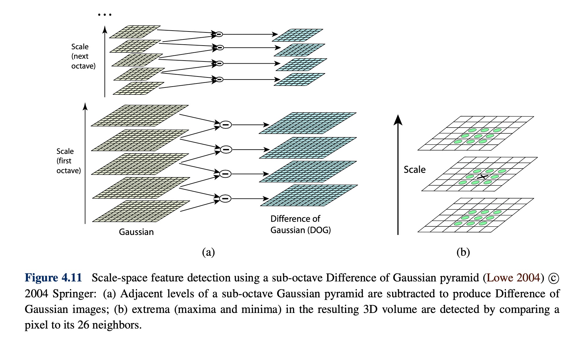
Early investigations into scale selection were performed by Lindeberg (1993; 1998b), who first proposed using extrema in the Laplacian of Gaussian (LoG) function as interest point locations. Based on this work, Lowe (2004) proposed computing a set of sub-octave Difference of Gaussian filters, looking for 3D (space+scale) maxima in the resulting structure (Figure 4.11b), and then computing a sub-pixel space+scale location using a quadratic fit (Brown and Lowe 2002). The number of sub-octave levels was determined, after careful empirical investigation, to be three, which corresponds to a quarter-octave pyramid, which is the same as used by Triggs (2004).

As with the Harris operator, pixels where there is strong asymmetry in the local curvature of the indicator function (in this case, the DoG) are rejected. This is implemented by first computing the local Hessian of the difference image D.
$H = \begin{bmatrix}D_{xx} & D_{xy} \\ D_{xy} & D_{yy}\end{bmatrix}$ and then rejecting keypoints for which $\displaystyle \frac{Trace(H)^2}{Det(H)} > 10$

While Lowe’s Scale Invariant Feature Transform (SIFT) performs well in practice, it is not based on the same theoretical foundation of maximum spatial stability as the auto-correlation- based detectors. (In fact, its detection locations are often complementary to those produced by such techniques and can therefore be used in conjunction with these other approaches.).

In order to add a scale selection mechanism to the Harris corner detector, Mikolajczyk and Schmid (2004) evaluate the Laplacian of Gaussian function at each detected Harris point (in a multi-scale pyramid) and keep only those points for which the Laplacian is extremal (larger or smaller than both its coarser and finer-level values). An optional iterative refinement for both scale and position is also proposed and evaluated.

Rotational invariance and orientation estimation

In addition to dealing with scale changes, most image matching and object recognition algorithms need to deal with (at least) in-plane image rotation. One way to deal with this problem is to design descriptors that are rotationally invariant (Schmid and Mohr 1997), but such descriptors have poor discriminability, i.e. they map different looking patches to the same descriptor.

A better method is to estimate a dominant orientation at each detected keypoint. Once the local orientation and scale of a keypoint have been estimated, a scaled and oriented patch around the detected point can be extracted and used to form a feature descriptor

The simplest possible orientation estimate is the average gradient within a region around the keypoint. If a Gaussian weighting function is used (Brown, Szeliski, and Winder 2005), this average gradient is equivalent to a first-order steerable filter, i.e., it can be computed using an image convolution with the horizontal and vertical derivatives of Gaussian filter (Freeman and Adelson 1991). In order to make this estimate more reliable, it is usually preferable to use a larger aggregation window (Gaussian kernel size) than detection window (Brown, Szeliski, and Winder 2005).

Sometimes, however, the averaged (signed) gradient in a region can be small and therefore an unreliable indicator of orientation. A more reliable technique is to look at the histogram of orientations computed around the keypoint. Lowe (2004) computes a 36-bin histogram of edge orientations weighted by both gradient magnitude and Gaussian distance to the cen- ter, finds all peaks within 80% of the global maximum, and then computes a more accurate orientation estimate using a three-bin parabolic fit

Affine invariance

While scale and rotation invariance are highly desirable, for many applications such as wide baseline stereo matching (Pritchett and Zisserman 1998; Schaffalitzky and Zisserman 2002) or location recognition (Chum, Philbin, Sivic et al. 2007), full affine invariance is preferred.

Affine-invariant detectors not only respond at consistent locations after scale and orientation changes, they also respond consistently across affine deformations such as (local) perspective foreshortening.

To introduce affine invariance, several authors have proposed fitting an ellipse to the auto-correlation or Hessian matrix (using eigenvalue analysis) and then using the principal axes and ratios of this fit as the affine coordinate frame

Another important affine invariant region detector is the maximally stable extremal region (MSER) detector developed by Matas, Chum, Urban et al. (2004). To detect MSERs, binary regions are computed by thresholding the image at all possible gray levels (the technique therefore only works for grayscale images). This operation can be performed efficiently by first sorting all pixels by gray value and then incrementally adding pixels to each connected component as the threshold is changed (Niste ́r and Stewe ́nius 2008). As the threshold is changed, the area of each component (region) is monitored; regions whose rate of change of area with respect to the threshold is minimal are defined as maximally stable. Such regions are therefore invariant to both affine geometric and photometric (linear bias-gain or smooth monotonic) transformations. If desired, an affine coordinate frame can be fit to each detected region using its moment matrix.

Feature descriptors

After detecting features (keypoints), we must match them, i.e., we must determine which features come from corresponding locations in different images. In some situations, e.g., for video sequences (Shi and Tomasi 1994) or for stereo pairs that have been rectified (Zhang, Deriche, Faugeras et al. 1995; Loop and Zhang 1999; Scharstein and Szeliski 2002), the lo- cal motion around each feature point may be mostly translational. In this case, simple error metrics, such as the sum of squared differences or normalized cross-correlation, described in Section 8.1 can be used to directly compare the intensities in small patches around each feature point. Because feature points may not be exactly located, a more accurate matching score can be computed by performing incremental motion refinement as described in Section 8.1.3 but this can be time consuming and can sometimes even decrease perfor- mance (Brown, Szeliski, and Winder 2005).

In most cases, however, the local appearance of features will change in orientation and scale, and sometimes even undergo affine deformations. Extracting a local scale, orientation, or affine frame estimate and then using this to resample the patch before forming the feature descriptor is thus usually preferable

@(MOPS)[Bias and gain normalization]

Multi-scale oriented patches (MOPS) descriptors are formed using an 8 × 8 sampling of bias and gain normalized intensity values, with a sample spacing of five pixels relative to the detection scale, using a coarser level of the image pyramid to avoid aliasing. (Brown, Szeliski, and Winder 2005) c 2005 IEEE. This low frequency sampling gives the features some robustness to interest point location error and is achieved by sampling at a higher pyramid level than the detection scale.

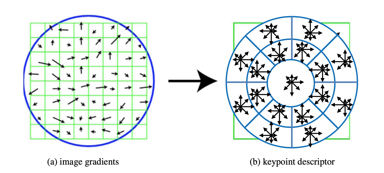
@(SIFT)[Scale invariant feature transform]

SIFT features are formed by computing the gradient at each pixel in a 16×16 window around the detected keypoint, using the appropriate level of the Gaussian pyramid at which the keypoint was detected. The gradient magnitudes are downweighted by a Gaussian fall-off function in order to reduce the influence of gradients far from the center, as these are more affected by small misregistrations.

@(variant of SIFT)[PCA-SIFT|SURF]

Ke and Sukthankar (2004) propose a simpler way to compute descriptors in- spired by SIFT; it computes the x and y (gradient) derivatives over a 39 × 39 patch and then reduces the resulting 3042-dimensional vector to 36 using principal component analysis (PCA) (Section 14.2.1 and Appendix A.1.2).
Another popular variant of SIFT is SURF (Bay, Tuytelaars, and Van Gool 2006), which uses box filters to approximate the derivatives and integrals used in SIFT.

@(Gradient location-orientation histogram)[GLOH]

This descriptor, developed by Miko- lajczyk and Schmid (2005), is a variant on SIFT that uses a log-polar binning structure instead of the four quadrants used by Lowe (2004). The spatial bins are of radius 6, 11, and 15, with eight angular bins (except for the central region), for a total of 17 spatial bins and 16 orientation bins. The 272-dimensional histogram is then projected onto a 128-dimensional descriptor using PCA trained on a large database. In their evaluation, Mikolajczyk and Schmid (2005) found that GLOH, which has the best performance overall, outperforms SIFT by a small margin.

@(Steerable filters)

Steerable filters are combinations of derivative of Gaus- sian filters that permit the rapid computation of even and odd (symmetric and anti-symmetric) edge-like and corner-like features at all possible orientations (Freeman and Adelson 1991). Because they use reasonably broad Gaussians, they too are somewhat insensitive to localiza- tion and orientation errors.

Feature matching

Once we have extracted features and their descriptors from two or more images, the next step is to establish some preliminary feature matches between these images. In this section, we divide this problem into two separate components.

• The first is to select a matching strategy, which determines which correspondences are passed on to the next stage for further process- ing.
• The second is to devise efficient data structures and algorithms to perform this matching as quickly as possible.

Matching strategy and error rates

we assume that the feature descriptors have been designed so that Euclidean (vector magnitude) distances in feature space can be directly used for ranking potential matches.

Efficient matching

Once we have decided on a matching strategy, we still need to search efficiently for poten- tial candidates. The simplest way to find all corresponding feature points is to compare all features against all other features in each pair of potentially matching images. Unfortunately, this is quadratic in the number of extracted features, which makes it impractical for most applications.

A better approach is to devise an indexing structure, such as a multi-dimensional search tree or a hash table, to rapidly search for features near a given feature. Such indexing struc- tures can either be built for each image independently or globally for all the images in a given database, which can potentially be faster, since it removes the need to it- erate over each image.

Feature match verification and densification

Once we have some hypothetical (putative) matches, we can often use geometric alignment to verify which matches are inliers and which ones are outliers.

Eg. if we expect the whole image to be translated or rotated in the matching view, we can fit a global geometric transform and keep only those feature matches that are sufficiently close to this estimated transformation. The process of selecting a small set of seed matches and then verifying a larger set is often called random sampling

Feature tracking

An alternative to independently finding features in all candidate images and then matching them is to find a set of likely feature locations in a first image and to then search for their corresponding locations in subsequent images.

This kind of detect then track approach is more widely used for video tracking applications, where the expected amount of motion and appearance deformation between adjacent frames is expected to be small.

The process of selecting good features to track is closely related to selecting good features for more general recognition applications. In practice, regions containing high gradients in both directions, i.e., which have high eigenvalues in the auto-correlation matrix (4.8), provide stable locations at which to find correspondences (Shi and Tomasi 1994).

One of the newest developments in feature tracking is the use of learning algorithms to build special-purpose recognizers to rapidly search for matching features anywhere in an image

Application: Performance-driven animation

One of the most compelling applications of fast feature tracking is performance-driven an- imation, i.e., the interactive deformation of a 3D graphics model based on tracking a user’s motions. See more detail Performance-driven animation

Use this technology in emoji field will be amazing

Edges

Edge detection

Qualitatively, edges occur at boundaries between regions of different color, intensity, or texture. Unfortunately, segmenting an image into coherent regions is a difficult task. Often, it is preferable to detect edges using only purely local information.

Under such conditions, a reasonable approach is to define an edge as a location of rapid intensity variation. Edges occur at locations of steep slopes, or equivalently, in regions of closely packed contour lines

A mathematical way to define the slope and direction of a surface is through its gradient,

$\displaystyle J(x) = \nabla I(x) = (\frac{\partial I}{\partial x}, \frac{\partial I}{\partial y})(x) \tag{2.0.5}$

The local gradient vector $J$ points in the direction of steepest ascent in the intensity function. Its magnitude is an indication of the slope or strength of the variation, while its orientation points in a direction perpendicular to the local contour.

Unfortunately, taking image derivatives accentuates high frequencies and hence amplifies noise, since the proportion of noise to signal is larger at high frequencies. It is therefore prudent to smooth the image with a low-pass filter prior to computing the gradient. Because we would like the response of our edge detector to be independent of orientation, a circularly symmetric smoothing filter is desirable.

Because differentiation is a linear operation, it commutes with other linear filtering operations. The gradient of the smoothed image can therefore be written as

$\displaystyle J_\sigma(x) = \nabla[G_\sigma(x) * I(x)] = [\nabla G_\sigma](x) * I(x) \tag{2.0.6}$

We can convolve the image with the horizontal and vertical derivatives of the Gaussian kernel function

$\nabla G_\sigma(x) = (\frac{\partial G_\sigma}{\partial x}, \frac{\partial G_\sigma}{\partial y})(x) = [-x -y]\frac{1}{\sigma^3}exp\bigg ( -\frac{x^2 + y^2}{2\sigma^2} \bigg ) \tag{2.0.7}$

For many applications, however, we wish to thin such a continuous gradient image to only return isolated edges, i.e., as single pixels at discrete locations along the edge contours. This can be achieved by looking for maxima in the edge strength (gradient magnitude) in a direction perpendicular to the edge orientation, i.e., along the gradient direction.

Finding this maximum corresponds to taking a directional derivative of the strength field in the direction of the gradient and then looking for zero crossings. The desired directional derivative is equivalent to the dot product between a second gradient operator and the results of the first

$S_\sigma(x) = \nabla \cdot J_\sigma(x) = [\nabla^2 G_\sigma](x) * I(x)$

The gradient operator dot product with the gradient is called the Laplacian. The convolution kernel

$\nabla^2 G_\sigma(x) = \frac{1}{\sigma^3}\bigg( 2 - \frac{x^2 + y^2}{2\sigma^2}\bigg )exp\bigg ( -\frac{x^2 + y^2}{2\sigma^2}\bigg ) \tag{2.0.8}$

is therefore called the Laplacian of Gaussian (LoG) kernel, which can be split into two separable parts

$\nabla^2 G_\sigma(x) = \frac{1}{\sigma^3}\bigg( 1 - \frac{x^2}{2\sigma^2}\bigg )G_\sigma(x)G_\sigma(y) + \frac{1}{\sigma^3}\bigg( 1 - \frac{y^2}{2\sigma^2}\bigg )G_\sigma(y)G_\sigma(x)$

which allows for a much more efficient implementation using separable filtering.

In practice, it is quite common to replace the Laplacian of Gaussian convolution with a Difference of Gaussian (DoG) computation, since the kernel shapes are qualitatively similar. This is especially convenient if a “Laplacian pyramid” has already been computed.

Edge linking

If the edges have been detected using zero crossings of some function, linking them up is straightforward, since adjacent edgels share common endpoints. Linking the edgels into chains involves picking up an unlinked edgel and following its neighbors in both directions.

Application: Edge editing and enhancement

Lines

While edges and general curves are suitable for describing the contours of natural objects, the man-made world is full of straight lines. Detecting and matching these lines can be useful in a variety of applications, including architectural modeling, pose estimation in urban environments, and the analysis of printed document layouts.

Successive approximation

Many techniques have been developed over the years to perform this approximation, which is also known as line simplification.

Hough transforms

The Hough transform is a well-known technique for having edges “vote” for plausible line locations.
procedure Hough$(\{(x, y, \theta)\})$

1. Clear the accumulator array.
2. For each detected edgel at location $(x,y)$ and orientation $\theta = tan^{-1} \frac{n_y}{n_x}$, compute the value of $d = xn_x + yn_y$ and increment the accumulator corresponding to $(\theta, d)$.
3. Find the peaks in the accumulator corresponding to lines.
4. Optionally re-fit the lines to the constituent edgels.

Note that the original formulation of the Hough transform, which assumed no knowledge of the edgel orientation θ, has an additional loop inside Step 2 that iterates over all possible values of θ and increments a whole series of accumulators.

Vanishing points

In many scenes, structurally important lines have the same vanishing point because they are parallel in 3D.
The first stage in my vanishing point detection algorithm uses a Hough transform to accumulate votes for likely vanishing point candidates. Using pairs of detected line segments to form candidate vanishing point locations.

Let $m_i$ and $m_j$ be the (unit norm) line equations for a pair of line segments and $l_i$ and $l_j$ be their corresponding segment lengths. The location of the corresponding vanishing point hypothesis can be computed as

$v_{ij} = m_i \times m_j \tag{2.0.9}$

and the corresponding weight set to

$w_ij = ||v_{ij}||l_il_j$

This has the desirable effect of downweighting (near-)collinear line segments and short line segments. The Hough space itself can either be represented using spherical coordinates or as a cube map.

Once the Hough accumulator space has been populated, peaks can be detected in a manner similar to that previously discussed for line detection. Given a set of candidate line segments that voted for a vanishing point, which can optionally be kept as a list at each Hough accu- mulator cell, I then use a robust least squares fit to estimate a more accurate location for each vanishing point.

Consider the relationship between the two line segment endpoints $\{p_{i0} , p_{i1}\}$ and the vanishing point $v$. The area A of the triangle given by these three points, which is the magnitude of their triple product

$\displaystyle A_i = |(p_{i0} \times p_{i1}) \cdot v| \tag{2.0.10}$

Assuming that the accuracy of a fitted line segment is proportional to its endpoint accuracy, this therefore serves as an optimal metric for how well a vanishing point fits a set of extracted lines. A robustified least squares estimate for the vanishing point can therefore be written as

$\epsilon = \sum_i\rho(A_i) = v^T\bigg(\sum_i \omega_i(A_i)m_im_i^T\bigg)v = v^TMv \tag{2.0.11}$

where $m_i = p_{i0} × p_{i1}$ is the segment line equation weighted by its length $l_i$, and $\omega_i = \rho′(A_i)/A_i$ is the influence of each robustified (reweighted) measurement on the final error.
Notice how this metric is closely related to the original formula for the pairwise weighted Hough transform accumulation step. The final desired value for $v$ is computed as the least eigenvector of $M$ .

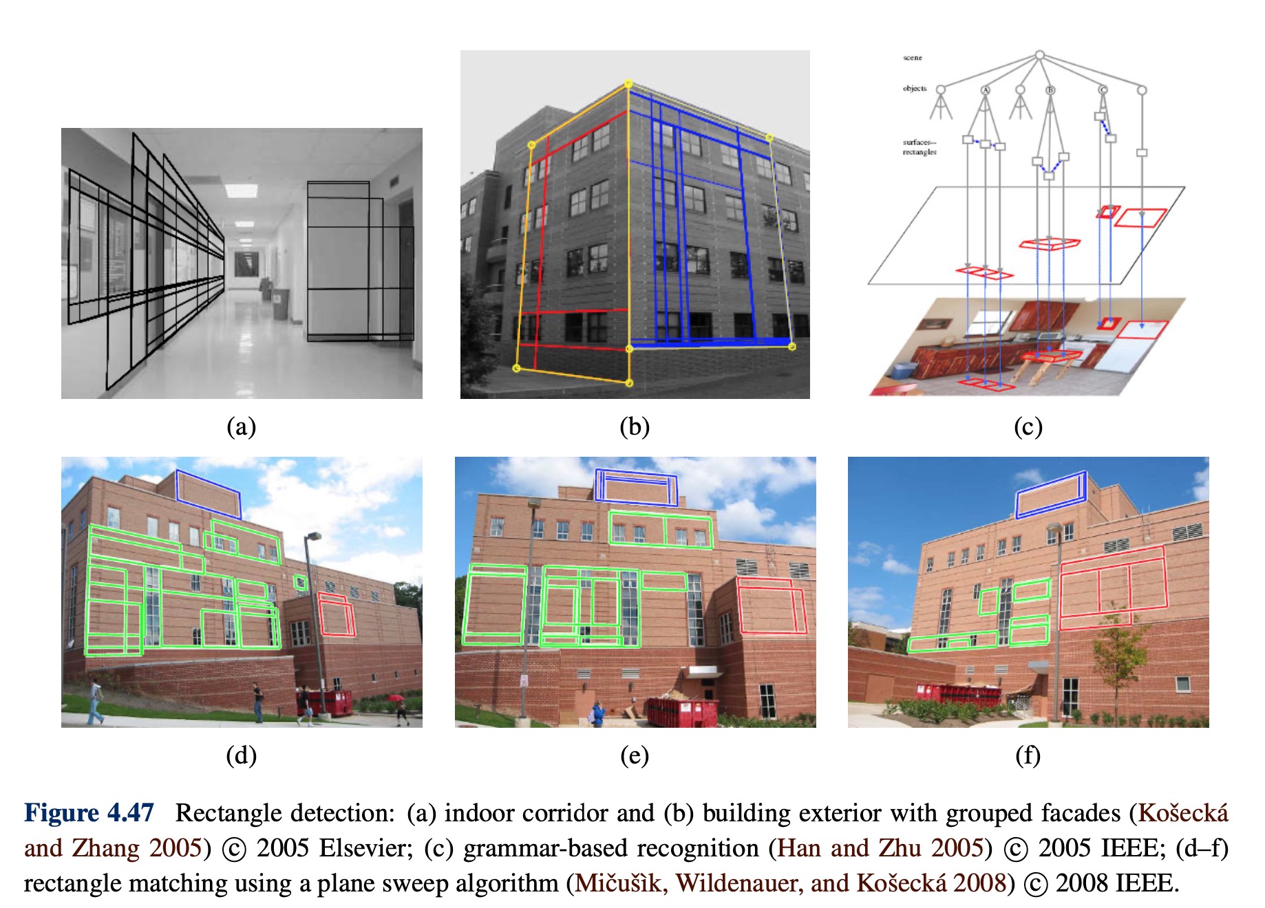
Application: Rectangle detection

the photoframe freezen can be amazing

Segmentation

Active contours

While lines, vanishing points, and rectangles are commonplace in the man-made world, curves corresponding to object boundaries are even more common, especially in the natural environment. In this section, we describe three related approaches to locating such boundary curves in images.

Snakes

Evolution: [Deep Snake for Real-Time Instance Segmentation]

Snakes are a two-dimensional generalization of the 1D energy-minimizing splines

$\epsilon_{int} = \int \alpha(s) ||f_s(s)||^2 + \beta(s)||f_{ss}(s)||^2ds\tag{3.0.1}$

where $s$ is the arc-length along the curve $f(s) = (x(s),y(s))$ and $\alpha(s)$ and $\beta(s)$ are first and second-order continuity weighting functions analogous to the $s(x, y)$ and $c(x, y)$ terms
We can discretize this energy by sampling the initial curve position evenly along its length to obtain

$E_{int} = \sum_i\alpha(i)||f(i + 1) -f(i)||^2 / h^2 + \beta(i)||f(i+1) - 2f(i) + f(i-1)||^2/h^4 \tag{3.0.2}$

where $h$ is the step size, which can be neglected if we resample the curve along its arc-length after each iteration.

In addition to this internal spline energy, a snake simultaneously minimizes external image-based and constraint-based potentials. The image-based potentials are the sum of sev- eral terms

$\epsilon_{image} = \omega_{line}\epsilon_{line} + \omega_{edge}\epsilon_{edge} + \omega_{term}\epsilon_{term} \tag{3.0.3}$

where the line term attracts the snake to dark ridges, the edge term attracts it to strong gradi- ents (edges), and the term term attracts it to line terminations. In practice, most systems only use the edge term, which can either be directly proportional to the image gradients

$E_{edge} = \sum_i -\left\| \nabla I (f(i))\right \|^2 \tag{3.0.4}$

or to a smoothed version of the image Laplacian

$E_{edge} = \sum_i -\left | (G_\sigma * \nabla^2 I) (f(i))\right |^2 \tag{3.0.5}$

People also sometimes extract edges and then use a distance map to the edges as an alternative to these two originally proposed potentials.

In interactive applications, a variety of user-placed constraints can also be added, e.g., attractive (spring) forces towards anchor points $d(i)$, then $E_{spring} = k_i\parallel f(i) - d(i) \parallel^2$. As the snakes evolve by minimiz- ing their energy, they often “wiggle” and “slither”.

Elastic nets and slippery springs

An interesting variant on snakes, first proposed by Durbin and Willshaw (1987) and later re-formulated in an energy-minimizing framework by Durbin, Szeliski, and Yuille (1989), is the elastic net formulation of the Traveling Salesman Problem (TSP).

Splines and shape priors

While snakes can be very good at capturing the fine and irregular detail in many real-world contours, they sometimes exhibit too many degrees of freedom, making it more likely that they can get trapped in local minima during their evolution.

One solution to this problem is to control the snake with fewer degrees of freedom through the use of B-spline approximations (Menet, Saint-Marc, and Medioni 1990b,a; Cipolla and Blake 1990). The resulting B-snake can be written as

$\displaystyle f(s) = \sum_kB_k(s)x_k$

or in discrete form as

$F = BX$

$F = \begin{bmatrix}f^T(0)\\ \vdots \\ f^T(N)\end{bmatrix}, B = \begin{bmatrix}B_0(s_0) & \cdots & B_K(s_0)\\ \vdots & \ddots & \vdots \\ B_0{s_N} & \cdots & B_K(s_N)\end{bmatrix}, X = \begin{bmatrix}x^T(0)\\ \vdots \\ x^T(K)\end{bmatrix}$

In a B-snake, because the snake is controlled by fewer degrees of freedom, there is less need for the internal smoothness forces used with the original snakes, although these can still be derived and implemented using finite element analysis, i.e., taking derivatives and integrals of the B-spline basis functions
In practice, it is more common to estimate a set of shape priors on the typical distribution of the control points $\{x_k\}$
A preferable approach is to estimate the joint covariance of all the points simultaneously. First, concatenate all of the point locations $\{x_k\}$ into a single vector $x$, e.g., by interleaving the $x$ and $y$ locations of each point. The distribution of these vectors across all training examples can be described with a mean $\bar x$ and a covariance

$C = \frac{1}{P}\sum_p(x_p - \bar x)(x_p - \bar x)^T \tag{3.0.6}$

where $x_p$ are the P training examples. Using eigenvalue analysis, which is also known as Principal Component Analysis (PCA), the covariance matrix can be written as

$C = \Phi\space diag(\lambda_0\cdots\lambda_{K-1})\space\Phi^T$

In most cases, the likely appearance of the points can be modeled using only a few eigen- vectors with the largest eigenvalues. The resulting point distribution model can be written as $x = \bar x + \hat\Phi b$, where $b$ is an $M\ll K$ element shape parameter vector and $\hat\Phi$ are the first m columns of $\Phi$
To constrain the shape parameters to reasonable values, we can use a quadratic penalty of the form

$E_{shape} = \frac{1}{2}b^T diag(\lambda_0\cdots\lambda_{M-1})b = \sum_m b_m^2/2\lambda_m \tag{3.0.7}$

In order to align a point distribution model with an image, each control point searches in a direction normal to the contour to find the most likely corresponding image edge point. These individual measurements can be combined with priors on the shape parameters (and, if desired, position, scale, and orientation parameters) to estimate a new set of parameters. The resulting Active Shape Model (ASM) can be iteratively minimized to fit images to non-rigidly deforming objects such as medical images or body parts such as hands (Cootes, Cooper, Taylor et al. 1995). The ASM can also be combined with a PCA analysis of the underlying gray-level distribution to create an Active Appearance Model (AAM)

Dynamic snakes and CONDENSATION

In many applications of active contours, the object of interest is being tracked from frame to frame as it deforms and evolves.

Scissors

Active contours allow a user to roughly specify a boundary of interest and have the system evolve the contour towards a more accurate location as well as track it over time. The results of this curve evolution, however, may be unpredictable and may require additional user-based hints to achieve the desired result.
An alternative approach is to have the system optimize the contour in real time as the user is drawing

Level Sets

A limitation of active contours based on parametric curves of the form $f(s)$, e.g., snakes, B-snakes, and CONDENSATION, is that it is challenging to change the topology of the curve as it evolves. Furthermore, if the shape changes dramatically, curve reparameterization may also be required.

An alternative representation for such closed contours is to use a level set, where the zero-crossing(s) of a characteristic function define the curve. Level sets evolve to fit and track objects of interest by modifying the underlying embedding function $\phi(x,y)$ instead of the curve $f(s)$

Application: Contour tracking and rotoscoping

Split and merge

Watershed

A technique related to thresholding, since it operates on a grayscale image, is watershed computation.This technique segments an image into several catchment basins, which are the regions of an image (interpreted as a height field or landscape) where rain would flow into the same lake. An efficient way to compute such regions is to start flooding the landscape at all of the local minima and to label ridges wherever differently evolving components meet. The whole algorithm can be implemented using a priority queue of pixels and breadth-first search

Unfortunately, watershed segmentation associates a unique region with each local minimum, which can lead to over-segmentation. Watershed segmentation is therefore often used as part of an interactive system, where the user first marks seed locations (with a click or a short stroke) that correspond to the centers of different desired components.

Region merging (agglomerative clustering)

Graph-based segmentation

Probabilistic aggregation

Mean shift and mode finding

Mean-shift and mode finding techniques, such as k-means and mixtures of Gaussians, model the feature vectors associated with each pixel (e.g., color and position) as samples from an unknown probability density function and then try to find clusters (modes) in this distribution.

Normalized cuts

Graph cuts and energy-based methods

Feature-based alignment

2D and 3D feature-based alignment

Feature-based alignment is the problem of estimating the motion between two or more sets of matched 2D or 3D points.

In this section, we restrict ourselves to global parametric trans- formations or higher order transformation for curved surfaces. Applications to non-rigid or elastic deformations are examined in later sections.

2D alignment using least squares

Given a set of matched feature points $\{(x_i , x_i' )\}$ and a planar parametric transformation of the form

$x' = f(x;p)\tag{4.0.1}$

Transform	Matrix	Parameters p	Jacobian J
translation	$\begin{bmatrix}1 & 0 & t_x\\0 & 1 & t_y\end{bmatrix}$	$(t_x, t_y)$	$\begin{bmatrix}1 & 0 \\ 0 & 1\end{bmatrix}$
Euclidean	$\begin{bmatrix}c_\theta & -s_\theta & t_x\\s_\theta & c_\theta & t_y\end{bmatrix}$	$(t_x, t_y, \theta)$	$\begin{bmatrix}1 & 0 & -s_\theta x - c_\theta y\\ 0 & 1 & c_\theta x - s_\theta y\end{bmatrix}$
similarity	$\begin{bmatrix}1 + a & -b & t_x\\b & 1+a & t_y\end{bmatrix}$	$(t_x, t_y, a, b)$	$\begin{bmatrix}1 & 0 & x & -y\\ 0 & 1 & y & x\end{bmatrix}$
affine	$\begin{bmatrix}1 + a_{00}& a_{01} & t_x\\a_{10} & 1 + a_{11} & t_y\end{bmatrix}$	$(t_x, t_y,a_{00}, a_{01}, a_{10}, a_{11})$	$\begin{bmatrix}1 & 0 & x & y & 0 & 0\\ 0 & 1 & 0 & 0 & x & y\end{bmatrix}$
projective	$\begin{bmatrix}1 + h_{00} & h_{01} & h_{02}\\h_{10} & 1 + h_{11} & h_{12}\\ h_{20} & h_{21} & 1\end{bmatrix}$	$(h_{00}, h_{01},\cdots,h_{21})$	see the part of Iterative algorithms$

how can we produce the best estimate of the motion parameters $p$? The usual way to do this is to use least squares, i.e., to minimize the sum of squared residuals

$E_{LS} = \sum_i\parallel r_i\parallel ^2 = \sum_i\parallel f(x_i;p) - x_i' \parallel ^2 \tag{4.0.2}$

$r_i = f(x_i;p) - x_i' = \hat x_i' - \tilde{x}_i'$

$r_i$ is the residual between the measured location $\hat x_i'$ and its corresponding current predicted location $\tilde{x}_i' = f(x_i;p)$
Many of the motion models i.e., translation, similarity, and affine, have a linear relationship between the amount of motion $\Delta x = x′ − x$ and the unknown parameters $p$, $\Delta x = x' - x = J(x)p$. where $J = \partial f/\partial p$ is the Jacobian of the transformation $f$ with respect to the motion parameters $p$. In this case, a simple linear regression (linear least squares problem) can be formulated as

$\begin{aligned} E_{LLS} &= \sum_i\parallel J(x_i)p - \Delta x_i \parallel ^2 \\ &= p^T\bigg[ \sum_iJ^T(x_i)J(x_i)\bigg]p - 2p^T\bigg[\sum_iJ^T(x_i)\Delta x_i\bigg] + \sum_i \parallel \Delta x_i \parallel ^2\\ &= p^TAp - 2p^Tb + c \end{aligned} \tag{4.0.3}$

The minimum can be found by solving the symmetric positive definite (SPD) system of $normal\space equations^2 \to Ap = b$, where $A = \sum_iJ^T(x_i)J(x_i)$ is called the Hessian and $b = \sum_i J^T(x_i)\Delta x_i$.

For the case of pure translation, the resulting equations have a particularly simple form, i.e., the translation is the average translation between corresponding points or, equivalently, the translation of the point centroids.

@(Uncertainty weighting)
The above least squares formulation assumes that all feature points are matched with the same accuracy. This is often not the case, since certain points may fall into more textured regions than others. If we associate a scalar variance estimate $\sigma_i^2$ with each correspondence, we can minimize the weighted least squares problem instead

$E_{WLS} = \sum_i\sigma_i^{-2}\parallel r_i\parallel ^2 \tag{4.0.4}$

A covariance estimate for patch-based matching can be obtained by multiplying the inverse of the patch Hessian $A_i$ with the per-pixel noise covariance $\sigma_n^2$. Weighting each squared residual by its inverse covariance $\varSigma_i^{-1} = \sigma_n^{-2}A_i$ (which is called the information matrix), we obtain

$E_{CWLS} = \sum_i\parallel r_i\parallel _{\sum_i^{-1}}^2 = \sum_ir_i^T\varSigma^{-1}r_i = \sum_i\sigma_n^{-2}r_i^TA_ir_i \tag{4.0.5}$

Application: Panography

One of the simplest (and most fun) applications of image alignment is a special form of image stitching called panography. In a panograph, images are translated and optionally rotated and scaled before being blended with simple averaging
In most of the examples seen on the Web, the images are aligned by hand for best artistic. However, it’s also possible to use feature matching and alignment techniques to perform the registration automatically.

Consider a simple translational model. We want all the corresponding features in different images to line up as best as possible. Let $t_j$ be the location of the $j_{th}$ image coordinate frame in the global composite frame and $x_{ij}$ be the location of the ith matched feature in the jth image. In order to align the images, we wish to minimize the least squares error

$E_{PLS} = \sum_{ij}\parallel (t_j + x_{ij}) - x_i \parallel ^2$

where $x_i$ is the consensus (average) position of feature $i$ in the global coordinate frame.

Iterative algorithms

While linear least squares is the simplest method for estimating parameters, most problems in computer vision do not have a simple linear relationship between the measurements and the unknowns. In this case, the resulting problem is called non-linear least squares or non-linear regression.

Pose estimation

Structure from motion